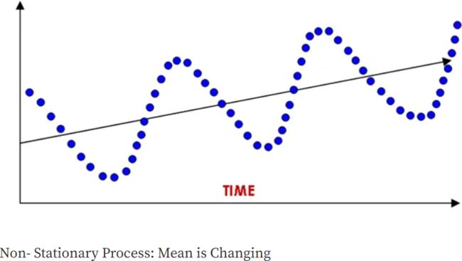
ts15_Forecast multiple seas_mSTL_make_subplot_rMSPE_UCM_date format_NeuralProphet_changepoint_StateS
Time series data can contain complex seasonality – for example, recorded hourly data can exhibit daily, weekly, and yearly seasonal patterns. With the rise of connected devices – for example, the Internet of Tings (IoT物联网:是指通过各种信息传感器、射频识别技术、全球定位系统、红外感应器、激光扫描器等各种装置与技术,实时采集任何需要监控、连接、互动的物体或过程,采集其声、光、热、电、力学、化学、生物、位置等各种需要的信息,通过各类可能的网络接入,实现物与物、物与人的泛在连接,实现对物品和过程的智能化感知、识别和管理。物联网是一个基于互联网、传统电信网等的信息承载体,它让所有能够被独立寻址的普通物理对象形成互联互通的网络) and sensors – data is being recorded more frequently. For example, if you examine classical time series datasets used in many research papers, many were smaller sets and recorded less frequently, such as annually or monthly. Such data contains one seasonal pattern. More recent datasets and research now use higher frequency data, recorded in hours or minutes.
Many of the algorithms we used in earlier chapters can work with seasonal time series. Still, they assume there is only one seasonal pattern, and their accuracy and results will suffer on more complex datasets.
In this chapter, you will explore new algorithms that can model a time series with multiple seasonality for forecasting and decomposing a time series into different components.
In this chapter, you will explore the following recipes:
- • Decomposing time series with multiple seasonal patterns using MSTL(Multiple Seasonal-Trend decomposition using Loess)
- • Forecasting with multiple seasonal patterns using the Unobserved Components Model (UCM)
- • Forecasting time series with multiple seasonal patterns using Prophet
- • Forecasting time series with multiple seasonal patterns using NeuralProphet
In this chapter, you will be using the Hourly Energy Consumption data from Kaggle
( https://www.kaggle.com/datasets/robikscube/hourly-energy-consumption ). Throughout the chapter, you will be working with the same energy dataset to observe how the different techniques compare.
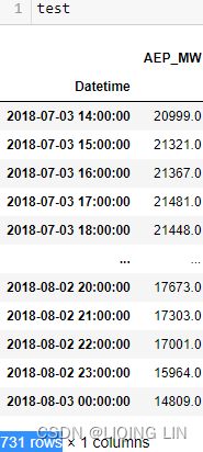
The recipes of this chapter will use one of these files, but feel free to explore the other ones. The files represent hourly energy consumption measured in megawatts (MW)兆瓦.
Read the AEP_hourly.csv file: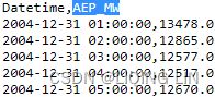 vs
vs
import pandas as pd

# from pathlib import Path

# folder = Path('./archive/')
# aep_file = folder.joinpath('AEP_hourly.csv')
# aep = pd.read_csv( aep_file,# American Electric Power
#                    index_col='Datetime',
#                    parse_dates=True
#                  )

base='https://raw.githubusercontent.com/PacktPublishing/Time-Series-Analysis-with-Python-Cookbook/main/datasets/Ch15/'

aep = pd.read_csv( base+'AEP_hourly.csv',# American Electric Power
                   index_col='Datetime',
                   parse_dates=True
                 )
aep 
aep.tail(n=26)
The time series is not in order and has some duplicate entries. The following are simple steps to clean up the data:
aep_cp = aep.copy(deep=True)
aep_cp.sort_index(inplace=True)
aep_cp = aep_cp.resample('H').max()
#Forward filling: ffill or pad ,
#uses the last value before the missing spot(s) and fills the gaps forward
aep_cp.ffill(inplace=True)
aep_cp
You should have a DataFrame with 121296 records of hourly energy consumption from October 2004 to August 2018 (around 15 years).
import matplotlib.pyplot as plt

aep_cp.plot(figsize=(12,4))
plt.show()
Understanding state-space models
In this chapter, you will see references to state-space models. In ts10_Univariate TS模型_circle mark pAcf_ETS_unpack product_darts_bokeh band interval_ljungbox_AIC_BIC_LIQING LIN的博客-CSDN博客ts10_2Univariate TS模型_pAcf_bokeh_AIC_BIC_combine seasonal_decompose twinx ylabel_bold partial title_LIQING LIN的博客-CSDN博客_first-order diff, Building Univariate Time Series Models Using Statistical Methods, you were introduced to exponential smoothing (Holt-Winters) and ARIMA-type models. Before defining what state-space models are, I want to point out that these models can be represented in a state-space formulation.
Each model consists of a measurement equation that describes the observed data, and some state equations that describe how the unobserved components or states (level, trend, seasonal) change over time. Hence, these are referred to as state space models.
State-Space Models (SSM) have their roots in the field of engineering (more specifically control engineering) and offer a generic/dʒəˈnerɪk/通用的 approach to modeling dynamic systems and how they evolve over time及其随时间演化的方式. In addition, SSMs are widely used in other fields, such as economics, neuroscience神经科学, electrical engineering, and other disciplines.
In time series data, the central idea behind SSMs is that of latent variables, also called states, which are continuous and sequential through the time-space domain. For example, in a univariate time series, we have a response variable at time t; this is the observed value termed ![]() , which depends on the true variable(independent variable) termed
, which depends on the true variable(independent variable) termed ![]() . The
. The ![]() variable is the latent variable that we are interested in estimating – which is either unobserved or cannot be measured. In state space, we have an underlying state that we cannot measure directly (unobserved). An SSM provides a system of equations to estimate these unobserved states from the observed values and is represented mathematically in a vector-matrix form. In general, there are two equations – a state equation and an observed equation. One key aspect of their popularity is their flexibility and ability to work with complex time series data that can be multivariate, non-stationary, non-linear, or contain multiple seasonality, gaps, or irregularities不规则性.
variable is the latent variable that we are interested in estimating – which is either unobserved or cannot be measured. In state space, we have an underlying state that we cannot measure directly (unobserved). An SSM provides a system of equations to estimate these unobserved states from the observed values and is represented mathematically in a vector-matrix form. In general, there are two equations – a state equation and an observed equation. One key aspect of their popularity is their flexibility and ability to work with complex time series data that can be multivariate, non-stationary, non-linear, or contain multiple seasonality, gaps, or irregularities不规则性.
In addition, SSMs can be generalized and come in various forms, several of which make use of Kalman filters (Kalman recursions). The benefit of using SSMs in time series data is that they are used in filtering, smoothing, or forecasting, as you will explore in the different recipes of this chapter.
Kalman Filters
The Kalman filter is an algorithm for extracting signals from data that is either noisy or contains incomplete measurements包含不完整测量值. The premise behind Kalman filters is that not every state within a system is directly observable; instead, we can estimate the state indirectly, using observations that may be contaminated, incomplete, or noisy.
For example, sensor devices produce time series data known to be incomplete due to interruptions or unreliable due to noise. Kalman filters are excellent when working with time series data containing a considerable signal-to-noise ratio, as they work on smoothing and denoising the data to make it more reliable.
Decomposing time series with multiple seasonal patterns using MSTL
The Decomposing time series data recipe in ts9_annot_arrow_hvplot PyViz interacti_bokeh_STL_seasonal_decomp_HodrickP_KPSS_F-stati_Box-Cox_Ljung_LIQING LIN的博客-CSDN博客, Exploratory Data Analysis and Diagnosis, introduced the concept of time series decomposition. In those examples, the time series had one seasonal pattern, and you were able to decompose it into three main parts – trend, seasonal pattern, and residual (remainder). In the recipe, you explored the seasonal_decompose function and the STL class (Seasonal-Trend decomposition using Loess) from statsmodels.
Recall, in an additive model(Y[t] = T[t] + S[t] + e[t]), your time series is reconstructed by the following equation:
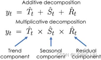
The additive decomposition is the most appropriate if the magnitude of the seasonal fluctuations季节性波动的幅度, or the variation around the trend-cycle,围绕趋势周期的变化 does not vary with the level of the time series.
Here, ![]() ,
, ![]() ,
, ![]() represent the seasonal, trend, and remainder components at time t respectively. But what about data with higher frequency – for example, IoT(Internet of Tings物联网) devices that can record data every minute or hour? Such data may exhibit multiple seasonal patterns.
represent the seasonal, trend, and remainder components at time t respectively. But what about data with higher frequency – for example, IoT(Internet of Tings物联网) devices that can record data every minute or hour? Such data may exhibit multiple seasonal patterns.
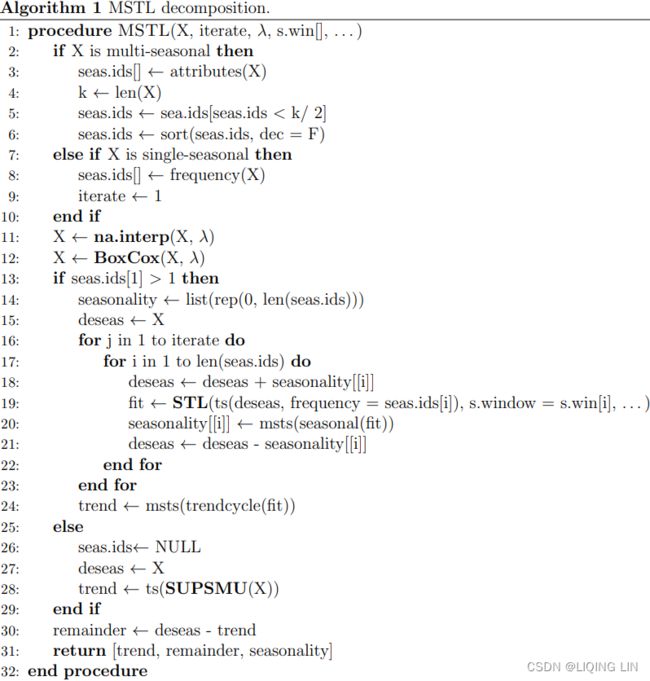
Given the limitations of traditional seasonal decomposition approaches, a new approach for decomposing time series with multiple seasonality was introduced in a paper published by Bandara, Hyndman, and Bergmeir, titled MSTL(Multiple Seasonal-Trend decomposition using Loess): A Seasonal-Trend Decomposition Algorithm for Time Series with Multiple Seasonal Patterns. The paper was published in July 2021, which you can read here: https://arxiv.org/pdf/2107.13462.pdf .
Multiple STL Decomposition (MSTL) is an extension of the STL algorithm and similarly is an additive decomposition, but it extends the equation to include multiple seasonal components and not just one:![]()

Here, n represents the number of seasonal cycles present in ![]() . The algorithm iteratively fits the STL decomposition for each seasonal cycle (frequency identified) to get the decomposed seasonal components –
. The algorithm iteratively fits the STL decomposition for each seasonal cycle (frequency identified) to get the decomposed seasonal components – ![]() . Once the iterative process for each seasonal cycle is completed, the trend component is estimated. If the time series does not have any seasonal components, MSTL will only estimate the trend.https://towardsdatascience.com/multi-seasonal-time-series-decomposition-using-mstl-in-python-136630e67530
. Once the iterative process for each seasonal cycle is completed, the trend component is estimated. If the time series does not have any seasonal components, MSTL will only estimate the trend.https://towardsdatascience.com/multi-seasonal-time-series-decomposition-using-mstl-in-python-136630e67530
The parameter iterate in MSTL defaults to iterate=2 , which is the number of iterations the algorithm uses to estimate the seasonal components. At each iteration, the algorithm applies the STL algorithm to estimate the seasonal component for each seasonal period identifed.
https://arxiv.org/pdf/2107.13462.pdf
statsmodels.tsa.stl.mstl — statsmodels
STl(Seasonal-Trend decomposition procedure based on Loess):https://www.wessa.net/download/stl.pdf
https://www.cnblogs.com/en-heng/p/7390310.html
statsmodels/_stl.pyx at main · statsmodels/statsmodels · GitHub
from statsmodels.tsa.tsatools import freq_to_period
from pandas.tseries.frequencies import to_offset
from statsmodels import tools

def test_freq_to_period():
    freqs = ['A', 'AS-MAR', 'Q', 'QS', 'QS-APR', 'W', 'W-MON', 'B']
    expected = [1, 1, 4, 4, 4, 52, 52, 52]
    for i, j in zip(freqs, expected):
        print(freq_to_period(i)==j)
        print(freq_to_period(to_offset(i))==j)

test_freq_to_period() ![]()

import numpy as np

n=2 # since there exists daily and week patterns
7 + 4 * np.arange(1, n+1, 1)
windows: ![]() <==
<==![]()
windows : Length of the seasonal smoothers for each corresponding period
import warnings
import numpy as np
import pandas as pd
from scipy.stats import boxcox

from statsmodels.tsa.seasonal import STL
from statsmodels.tsa.tsatools import freq_to_period

class MSTL:
    """
    MSTL(endog, periods=None, windows=None, lmbda=None, iterate=2,
         stl_kwargs=None)

    Season-Trend decomposition using LOESS for multiple seasonalities.

    Parameters
    ----------
    endog : array_like
        Data to be decomposed. Must be squeezable to 1-d.
    periods : {int, array_like, None}, optional
        Periodicity of the seasonal components. If None and endog is a pandas
        Series or DataFrame, attempts to determine from endog. If endog is a
        ndarray, periods must be provided.
    windows : {int, array_like, None}, optional
        Length of the seasonal smoothers for each corresponding period.
        Must be an odd integer, and should normally be >= 7 (default). If None
        then default values determined using 7 + 4 * np.arange(1, n + 1, 1)
        where n is number of seasonal components.
        # if n=1 : When you used STL,
        # you provided seasonal=13=windows[i] because the data has an annual seasonal effect.
    lmbda : {float, str, None}, optional
        The lambda parameter for the Box-Cox transform to be applied to `endog`
        prior to decomposition. If None, no transform is applied. If "auto", a
        value will be estimated that maximizes the log-likelihood function.
    iterate : int, optional
        Number of iterations to use to refine the seasonal component.
    stl_kwargs: dict, optional
        Arguments to pass to STL.

    See Also
    --------
    statsmodels.tsa.seasonal.STL

    References
    ----------
    .. [1] K. Bandura, R.J. Hyndman, and C. Bergmeir (2021)
        MSTL: A Seasonal-Trend Decomposition Algorithm for Time Series with
        Multiple Seasonal Patterns. arXiv preprint arXiv:2107.13462.

    Examples
    --------
    Start by creating a toy dataset with hourly frequency and multiple seasonal
    components.

    >>> import numpy as np
    >>> import matplotlib.pyplot as plt
    >>> import pandas as pd
    >>> pd.plotting.register_matplotlib_converters()
    >>> np.random.seed(0)
    >>> t = np.arange(1, 1000)
    >>> trend = 0.0001 * t ** 2 + 100
    >>> daily_seasonality = 5 * np.sin(2 * np.pi * t / 24)
    >>> weekly_seasonality = 10 * np.sin(2 * np.pi * t / (24 * 7))
    >>> noise = np.random.randn(len(t))
    >>> y = trend + daily_seasonality + weekly_seasonality + noise
    >>> index = pd.date_range(start='2000-01-01', periods=len(t), freq='H')
    >>> data = pd.DataFrame(data=y, index=index)

    Use MSTL to decompose the time series into two seasonal components
    with periods 24 (daily seasonality) and 24*7 (weekly seasonality).

    >>> from statsmodels.tsa.seasonal import MSTL
    ###       MSTL(aep_cp, periods=(day, week) ) # freq='H'
    >>> res = MSTL( data, periods=(24, 24*7) ).fit()
    >>> res.plot()
    >>> plt.tight_layout()
    >>> plt.show()

    .. plot:: plots/mstl_plot.py
    """
    def _infer_period(self):
        freq = None
        if isinstance( self.endog, (pd.Series, pd.DataFrame) ): # 8: seas.ids[] ← frequency(X)
            freq = getattr( self.endog.index, "inferred_freq", None ) # freq='H'
        if freq is None:
            raise ValueError("Unable to determine period from endog")
        period = freq_to_period(freq)                                 # period=24
        return period                           # 3. seas.ids[] ← attributes(X)

    def _process_periods(self, periods):
        if periods is None:
            periods = ( self._infer_period(), ) # 3. seas.ids[] ← attributes(X)
        elif isinstance( periods, int ):
            periods = ( periods, )
        else:
            pass
        return periods

    @staticmethod
    def _default_seasonal_windows(n):
        return tuple( 7 + 4 * i
                      for i in range(1, n + 1)
                    )  # See [1]

    def _process_windows(self, windows,num_seasons ) :
        if windows is None:
            windows = self._default_seasonal_windows(num_seasons)
        elif isinstance(windows, int):
            windows = (windows,)
        else:
            pass
        return windows

    @staticmethod
    def _sort_periods_and_windows( periods, windows ):
        if len(periods) != len(windows):
            raise ValueError("Periods and windows must have same length")
        periods, windows = zip( *sorted( zip(periods, windows) ) )
        return periods, windows

    def _process_periods_and_windows( self,
                                      periods,
                                      windows,
                                    ):
        periods = self._process_periods(periods)

        if windows:
            windows = self._process_windows( windows, num_seasons=len(periods) )
            periods, windows = self._sort_periods_and_windows( periods, windows )
        else:
            windows = self._process_windows( windows, num_seasons=len(periods) )
            periods = sorted(periods)    # 6. : seas.ids ← sort(seas.ids, dec = F)

        if len(periods) != len(windows):
            raise ValueError("Periods and windows must have same length")

        # Remove long periods from decomposition
        if any( period >= self.nobs / 2
                for period in periods
              ):                         # 2: if X is multi-seasonal then
            warnings.warn( "A period(s) is larger than half the length of time series."
                           " Removing these period(s)."
                         )
            periods = tuple( period
                             for period in periods
                                if period < self.nobs / 2
                           )             # 5: seas.ids ← sea.ids[seas.ids < k/ 2]
            windows = windows[: len(periods)]

        return periods, windows

    @staticmethod
    def _to_1d_array(x):
        y = np.ascontiguousarray( np.squeeze( np.asarray(x) ), dtype=np.double )
        # Return a contiguous array (ndim >= 1) in memory (C order)
        # (C order): Row-major order: row by row
        if y.ndim != 1:
            raise ValueError("y must be a 1d array")
        return y

    def __init__( self, endog, *,
                  periods= None,
                  windows= None,
                  lmbda= None,
                  iterate =2,
                  stl_kwargs= None,
                ):
        self.endog = endog
        self._y = self._to_1d_array(endog) # Data to be decomposed
        self.nobs = self._y.shape[0]     # 4: k ← len(X)
        self.lmbda = lmbda
        self.periods, self.windows = self._process_periods_and_windows(periods,
                                                                       windows
                                                                      )
        self.iterate = iterate
        self._stl_kwargs = self._remove_overloaded_stl_kwargs(
                                    stl_kwargs if stl_kwargs else {}
                           )
    def fit(self):
        """
        Estimate a trend component, multiple seasonal components, and a
        residual component.

        Returns
        -------
        DecomposeResult
            Estimation results.
        """
        num_seasons = len(self.periods)
        iterate = 1 if num_seasons == 1 else self.iterate
        #9:iterate ← 1  # 7: else if X is single-seasonal then
        # Box Cox
        if self.lmbda == "auto":         # 12: X ← BoxCox(X, λ)
            # https://blog.csdn.net/Linli522362242/article/details/127737895
            # Box-Cox allows us to make the data both normal and homoskedastic
            y, lmbda = boxcox(self._y, lmbda=None) # If the lmbda parameter is None,
            # the second returned argument is the lmbda that maximizes the log-likelihood function.
            self.est_lmbda = lmbda
        elif self.lmbda:
            # Return a dataset transformed by a Box-Cox power transformation.
            y = boxcox(self._y, lmbda=self.lmbda)
        else:
            y = self._y

        # Get STL fit params
        stl_inner_iter = self._stl_kwargs.pop("inner_iter", None)
        stl_outer_iter = self._stl_kwargs.pop("outer_iter", None)

        # Iterate over each seasonal component to extract seasonalities
                                         # 14: seasonality ← list(rep(0, len(seas.ids)))
        seasonal = np.zeros(shape=(num_seasons, self.nobs))
        deseas = y                       # 15: deseas ← X
        # Y_t = S_t^1 + S_t^2 + ... + S_t^n + T_t + R_t
        for _ in range(iterate):         # 16: for j in 1 to iterate do
            for i in range(num_seasons): # 17: for i in 1 to len(seas.ids) do
                deseas = deseas + seasonal[i] # 18: deseas ← deseas + seasonality[[i]]
                # 19: fit ← STL(ts(deseas, frequency = seas.ids[i]), s.window = s.win[i], . . . )
                res = STL( endog=deseas,
                           period=self.periods[i],
                           seasonal=self.windows[i],
                           **self._stl_kwargs,
                         ).fit(inner_iter=stl_inner_iter,
                               outer_iter=stl_outer_iter
                              )
                seasonal[i] = res.seasonal    # 20: seasonality[[i]] ← msts(seasonal(fit))
                deseas = deseas - seasonal[i] # 21: deseas ← deseas - seasonality[[i]]

        seasonal = np.squeeze(seasonal.T)
        # statsmodels.tsa.seasonal.DecomposeResult
        trend = res.trend                     # 24: trend ← msts(trendcycle(fit))
        rw = res.weights # The weights used to reduce outlier influence.
        resid = deseas - trend                # 30: remainder ← deseas - trend

        # Return pandas if endog is pandas
        if isinstance(self.endog, (pd.Series, pd.DataFrame)):
            index = self.endog.index
            y = pd.Series(y, index=index, name="observed")
            trend = pd.Series(trend, index=index, name="trend")
            resid = pd.Series(resid, index=index, name="resid")
            rw = pd.Series(rw, index=index, name="robust_weight")
            cols = [f"seasonal_{period}" for period in self.periods]
            if seasonal.ndim == 1:
                seasonal = pd.Series(seasonal, index=index, name="seasonal")
            else:
                seasonal = pd.DataFrame(seasonal, index=index, columns=cols)

        # Avoid circular imports
        from statsmodels.tsa.seasonal import DecomposeResult

        return DecomposeResult(y, seasonal, trend, resid, rw)

    def __str__(self):
        return (
            "MSTL(endog,"
            f" periods={self.periods},"
            f" windows={self.windows},"
            f" lmbda={self.lmbda},"
            f" iterate={self.iterate})"
        )

    @staticmethod
    def _remove_overloaded_stl_kwargs(stl_kwargs):
        args = ["endog", "period", "seasonal"]
        for arg in args:
            stl_kwargs.pop(arg, None)
        return stl_kwargs
In Python, the algorithm is implemented in statsmodel as the MSTL class. At the time of writing, the MSTL class is only available in the development version of statsmodels, which is the 0.14.0 version. The current stable version is 0.13.2 . The following instructions will show you how to install the development version.
pip install git+https://github.com/statsmodels/statsmodelsGenerally, high-frequency data exhibits multiple seasonal patterns. For example, hourly time series data can have a daily, weekly, and annual pattern. You will start by importing the MSTL class from statsmodels and explore how to decompose the energy consumption time series.
2. Create four variables to hold values for day, week, month, and year calculations; this way, you can reference these variables. For example, since the data is hourly, a day is represented as 24 hours and a week as 24 X 7 , or simply day X 7 :
day = 24
week = day*7
month = round(week*4.35)
year = round(month*12)

print(f'''
day = {day} hours
week = {week} hours
month = {month} hours
year = {year} hours
''')

3. Start by providing the different seasonal cycles you suspect – for example, a daily and weekly seasonal pattern:
Since the data's frequency is hourly, a daily pattern is observed every 24 hours(since freq='H') and weekly every 24 x 7 or 168 hours.
4. Use the fit method to fit the model. The algorithm will first estimate the two seasonal periods ( ![]() ), then the trend, and finally, the remainder:
), then the trend, and finally, the remainder:
#mstl = MSTL(aep_cp, periods=(day, week) )
mstl = MSTL(aep_cp, periods=(24, 24*7))# 24 hours since freq='H' in the ts dataset
results_mstl = mstl.fit()
5. The results object is an instance of the DecomposeResult class, which gives access to the seasonal , trend , and resid attributes. The seasonal attribute will display a DataFrame with two columns labeled seasonal_24 and seasonal_168.
results_mstl.seasonal
You can plot each attribute individually or use the plot method to plot all the components:
plt.rcParams["figure.figsize"] = [10, 8]

ax=results_mstl.plot()
ax.tight_layout()
plt.show()
fig, axes = plt.subplots(3+len(results_mstl.seasonal.columns), 1,
                         figsize=(10,8)
                        )
results_mstl.observed.plot( ax=axes[0],
                           title=results_mstl.observed.name.capitalize()
                          )
results_mstl.trend.plot( ax=axes[1],
                         ylabel=results_mstl.trend.name.capitalize()
                       )
for i in range( len(results_mstl.seasonal.columns) ):
    results_mstl.seasonal[results_mstl.seasonal.columns[i]].plot(ax=axes[2+i],
                                                                 ylabel=results_mstl.seasonal.columns[i].capitalize()
                                                                )
results_mstl.resid.plot( ax=axes[-1], ylabel=results_mstl.resid.name.capitalize(),
                         marker='o', linewidth=0
                       )

plt.subplots_adjust(hspace = 0.3)
plt.show()
The preceding code will produce five subplots for the observed trend , seasonal_24 (daily), seasonal_168 (weekly), and resid (the remainder) respectively:
 Figure 15.1 – The MSTL decomposition plot for the energy consumption data
fig, axes = plt.subplots(3+len(results_mstl.seasonal.columns), 1,
                         figsize=(10,8)
                        )
results_mstl.observed.plot( ax=axes[0], title=results_mstl.observed.name.capitalize() )
results_mstl.trend.plot( ax=axes[1], ylabel=results_mstl.trend.name.capitalize() )
for i in range( len(results_mstl.seasonal.columns) ):
    results_mstl.seasonal[results_mstl.seasonal.columns[i]].plot(ax=axes[2+i],
                                                                 ylabel=results_mstl.seasonal.columns[i].capitalize()
                                                                )
results_mstl.resid.plot( ax=axes[-1], ylabel=results_mstl.resid.name.capitalize() )

axes[-1].axhline(y=np.mean(results_mstl.resid), color='k', linestyle='--')

plt.subplots_adjust(hspace = 0.3)
plt.show()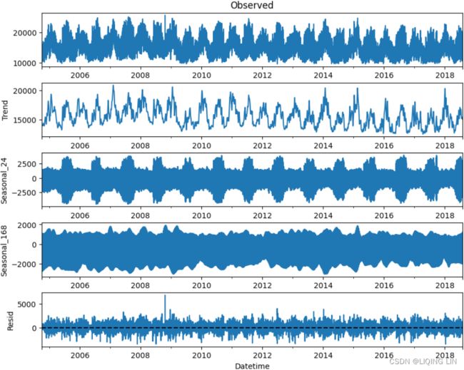
Given the amount of data, it is hard to observe the extracted patterns. Slice the data to zoom in for a better visual perspective.
make_subplots:
Part 4. Interactive Graphing and Crossfiltering | Dash for Python Documentation | Plotly
import plotly.graph_objects as go
from plotly.subplots import make_subplots
def plotly_stl( results ):
#https://plotly.github.io/plotly.py-docs/plotly.subplots.html
fig = make_subplots( rows=3+len(results.seasonal.columns), cols=1,
shared_xaxes=False,
#subplot_titles=(results.observed.name.capitalize()),
)
precision = 2
customdataName=[results.observed.name.capitalize(),
results.trend.name.capitalize(),
results.seasonal.columns[0].capitalize(),
results.seasonal.columns[1].capitalize(),
results.resid.name.capitalize(),
]
customdata=np.stack((results.observed,
results.trend,
results.seasonal[results.seasonal.columns[0]],
results.seasonal[results.seasonal.columns[1]],
results.resid,
),
axis=-1
)
#print(customdata)
fig.append_trace( go.Scatter( name=customdataName[0],
mode ='lines',
x=results.observed.index,
y=results.observed,
line=dict(shape = 'linear', #color = 'blue', #'rgb(100, 10, 100)',
width = 2, #dash = 'dash'
),
customdata=customdata,
hovertemplate='
'.join(['Datetime: %{x:%Y-%m-%d:%h}',
''+customdataName[0]+''+f": %{{y:.{precision}f}}"+'',
customdataName[1] + ": %{customdata[1]:.2f}",
customdataName[2] + ": %{customdata[2]:.2f}",
customdataName[3] + ": %{customdata[3]:.2f}",
customdataName[4] + ": %{customdata[4]:.2f}",
'
'.join(['Datetime: %{x:%Y-%m-%d:%h}',
''+customdataName[1]+''+f": %{{y:.{precision}f}}"+'',
customdataName[0] + ": %{customdata[0]:.2f}",
customdataName[2] + ": %{customdata[2]:.2f}",
customdataName[3] + ": %{customdata[3]:.2f}",
customdataName[4] + ": %{customdata[4]:.2f}",
'
'.join(['Datetime: %{x:%Y-%m-%d:%h}',
''+customdataName[2+i]+''+f": %{{y:.{precision}f}}"+'',
customdataName[0] + ": %{customdata[0]:.2f}",
customdataName[1] + ": %{customdata[1]:.2f}",
customdataName[another] + f": %{{customdata[{another}]:.{precision}f}}",
customdataName[4] + ": %{customdata[4]:.2f}",
'
'.join(['Datetime: %{x:%Y-%m-%d:%h}',
''+customdataName[4]+''+f": %{{y:.{precision}f}}"+'',
customdataName[0] + ": %{customdata[0]:.2f}",
customdataName[1] + ": %{customdata[1]:.2f}",
customdataName[2] + ": %{customdata[2]:.2f}",
customdataName[3] + ": %{customdata[3]:.2f}",
'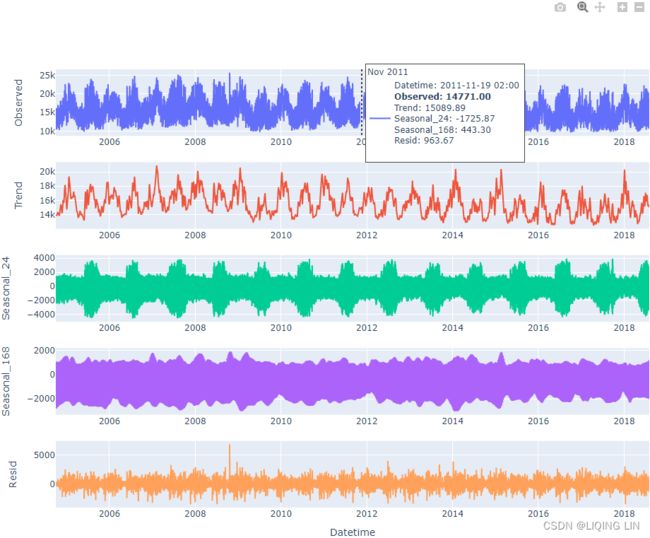
6. Generally, you would expect a daily pattern where energy consumption peaks during the day and declines at nighttime. Additionally, you would anticipate a weekly pattern where consumption is higher on weekdays compared to weekends when people travel or go outside more. An annual pattern is also expected, with higher energy consumption peaking in the summer than in other cooler months.
Slice the data and plot the components individually. Start with the daily seasonal pattern:
# mask = results.seasonal.index.month==7
fig, ax = plt.subplots( 2, 1, figsize=(10, 5) )
results_mstl.seasonal['seasonal_24'].loc['2016-01-04':'2016-01-06'].plot(ax=ax[0],
                                                                         title='Daily Seasonality in January'
                                                                        )
results_mstl.seasonal['seasonal_24'].loc['2016-07-04':'2016-07-06'].plot(ax=ax[1],
                                                                         title='Daily Seasonality in July'
                                                                        )
fig.tight_layout()
plt.show()
The preceding code will show two subplots – 3 days in January (Monday–Wednesday) and 3 days in July (Monday–Wednesday):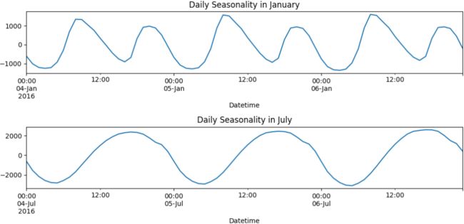
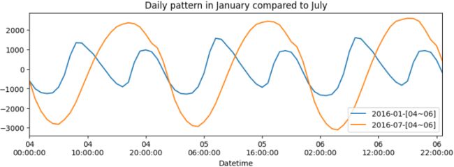
Figure 15.2 – Daily pattern in January compared to July
There is a repeating pattern of peaks during the day, which declines as it gets closer to the evening. Note that in the summertime, the daily pattern changes. For example, the daily pattern is similar in July, except the peak during the day is extended longer into later in the evening, possibly due to air conditioners being used at night before the weather cools down a little.
import matplotlib.ticker as ticker
from datetime import datetime

s24_1=results_mstl.seasonal['seasonal_24'].loc['2016-01-04':'2016-01-06'].index
s24_1_datetime=[]
s24_7=results_mstl.seasonal['seasonal_24'].loc['2016-07-04':'2016-07-06'].index
s24_7_datetime=[]

for i in range(len(s24_1)):
    s24_1_datetime.append( datetime.strftime(s24_1[i], '%d\n%H:%M:%S') )
    s24_7_datetime.append( datetime.strftime(s24_7[i], '%d\n%H:%M:%S') )

fig, ax = plt.subplots( 1, 1, figsize=(10, 3) )

ax.plot( s24_1_datetime,#np.arange(len(s24_1_datetime)),
         results_mstl.seasonal['seasonal_24'].loc['2016-01-04':'2016-01-06'].values,
         label=datetime.strftime(s24_1[i], '%Y-%m')+'-[04-06]'
        )
ax.plot( s24_7_datetime,#np.arange(len(s24_7_datetime)),
         results_mstl.seasonal['seasonal_24'].loc['2016-07-04':'2016-07-06'].values,
         label=datetime.strftime(s24_7[i], '%Y-%m')+'-[04-06]'
       )
ax.legend()

ax.xaxis.set_major_locator( ticker.MaxNLocator(8) )
ax.autoscale(enable=True, axis='x', tight=True)
ax.set_xlabel('Datetime')
ax.set_title('Daily pattern in January compared to July')
plt.show()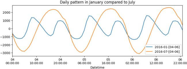
import matplotlib.ticker as ticker
from datetime import datetime

def plot_patterns(df,
                  startDate1, endDate1,
                  startDate7, endDate7,
                  title, xlabel, ylabel=None
                 ):
    df_1 = df.loc[startDate1:endDate1].index
    df_1_datetime=[]
    df_7 = df.loc[startDate7:endDate7].index
    df_7_datetime=[]

    for i in range(len(df_1)):
        df_1_datetime.append( datetime.strftime(df_1[i], '%d\n%H:%M:%S') )
        df_7_datetime.append( datetime.strftime(df_7[i], '%d\n%H:%M:%S') )

    fig, ax = plt.subplots( 1, 1, figsize=(10, 3) )

    ax.plot( df_1_datetime,#np.arange(len(s24_1_datetime)),
             df.loc[startDate1:endDate1].values,
             label=datetime.strftime(df_1[i], '%Y-%m') + '-[' + startDate1[-2:] +'~'+ endDate1[-2:] + ']'
           )
    ax.plot( df_7_datetime,#np.arange(len(s24_7_datetime)),
             df.loc[startDate7:endDate7].values,
             label=datetime.strftime(df_7[i], '%Y-%m') + '-[' + startDate7[-2:] +'~'+ endDate7[-2:] + ']'
           )
    ax.legend()

    ax.xaxis.set_major_locator( ticker.MaxNLocator(8) )
    ax.autoscale(enable=True, axis='x', tight=True)
    ax.set_xlabel(xlabel)
    ax.set_title(title)
    plt.show()

plot_patterns( results_mstl.seasonal[['seasonal_24']],
               '2016-01-04', '2016-01-06',
               '2016-07-04', '2016-07-06',
               title='Daily pattern in January compared to July',
               xlabel='Datetime',
             )
from datetime import datetime
s24_1=results_mstl.seasonal['seasonal_24'].loc['2016-01-04':'2016-01-06'].index
s24_1_datetime=[]
s24_7=results_mstl.seasonal['seasonal_24'].loc['2016-07-04':'2016-07-06'].index
s24_7_datetime=[]
for i in range(len(s24_1)):
s24_1_datetime.append( datetime.strftime(s24_1[i], '%d %H:%M:%S') )
s24_7_datetime.append( datetime.strftime(s24_7[i], '%d %H:%M:%S') )
layout=go.Layout(width=1000, height=500,
xaxis=dict(title='DateTime', color='black', tickangle=-30),
yaxis=dict(title='Energy Consumption', color='black'),
title=dict(text='Daily pattern in January compared to July',
x=0.5, y=0.9
),
)
fig = go.Figure(layout=layout)
# https://plotly.com/python/marker-style/#custom-marker-symbols
# circle-open-dot
# https://support.sisense.com/kb/en/article/changing-line-styling-plotly-python-and-r
fig.add_trace( go.Scatter( name=datetime.strftime(s24_1[i], '%Y-%m')+'-[04-06]',
mode ='lines', #marker_symbol='circle',
line=dict(shape = 'linear', color = 'blue',#'rgb(100, 10, 100)',
width = 2, #dash = 'dashdot'
),
x=s24_1_datetime,
y=results_mstl.seasonal['seasonal_24'].loc['2016-01-04':'2016-01-06'].values,
hovertemplate = 'energy: %{y:.1f}
from datetime import datetime
def plotly_patterns(df,
startDate1, endDate1,
startDate7, endDate7,
title, xlabel, ylabel=None,
legend_x=0, legend_y=1,
nticks=6, tickformat='%d %H:%M:%S',
):
df_1=df.loc[startDate1:endDate1].index
df_1_datetime=df.loc[startDate1:endDate1].index.strftime(tickformat)
df_7=df.loc[startDate7:endDate7].index
df_7_datetime=df.loc[startDate7:endDate7].index.strftime(tickformat)
layout=go.Layout(width=1000, height=500,
xaxis=dict(title=xlabel, color='black', tickangle=-30),
yaxis=dict(title=ylabel, color='black'),
title=dict(text=title,
x=0.5, y=0.9
),
)
fig = go.Figure(layout=layout)
# https://plotly.com/python/marker-style/#custom-marker-symbols
# circle-open-dot
# https://support.sisense.com/kb/en/article/changing-line-styling-plotly-python-and-r
fig.add_trace( go.Scatter( name=datetime.strftime(df_1[0], '%Y-%m') + '-[' + startDate1[-2:] +'~'+ endDate1[-2:] + ']',
mode ='lines', #marker_symbol='circle',
line=dict(shape = 'linear', color = 'blue',#'rgb(100, 10, 100)',
width = 2, #dash = 'dashdot'
),
x=df_1_datetime,
y=df.loc[startDate1:endDate1].values.reshape(-1),
hovertemplate = 'energy: %{y:.1f}

There is a repeating pattern of peaks during the day, which declines as it gets closer to the evening. Note that in the summertime, the daily pattern changes. For example, the daily pattern is similar in July, except the peak during the day is extended longer into later in the evening, possibly due to air conditioners being used at night before the weather cools down a little.
7. Perform a similar slice for the weekly seasonal pattern:
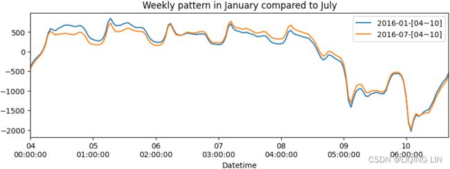
plot_patterns( results_mstl.seasonal[['seasonal_168']],
               '2016-01-04', '2016-01-10',
               '2016-07-04', '2016-07-10',
               title='Weekly pattern in January compared to July',
               xlabel='Datetime',
             )
The preceding code should produce a similar plot to Figure 15.2, displaying the entire first week in January 2016 (Monday–Sunday) and July 2016 (Monday–Sunday). There is a noticeable pattern of highs during weekdays that slowly decays during the weekend. During July, the sharper drop in the weekend周末降幅较大 is possibly due to people enjoying outdoor activities.
plotly_patterns( results_mstl.seasonal[['seasonal_168']],
                '2016-01-04', '2016-01-17',
                '2016-07-04', '2016-07-17',
                title='Weekly pattern in January compared to July',
                xlabel='Datetime',
                legend_x=0,legend_y=0,
                nticks=12, tickformat='%d(%A) %H:%M:%S'
               )
Overall, the results (from daily and weekly) suggest an annual influence indicative of an annual seasonal pattern. In the There's more section, you will explore how you can expose this annual pattern (to capture repeating patterns every July as an example).
n=2 # since there exists daily and week patterns
7 + 4 * np.arange(1, n+1, 1) ![]() <==
<==![]()
You will update windows to [121, 121] for each seasonal component in the following code. The default values for windows are [11, 15] . The default value for iterate is 2 , and you will update it to 4.
# mstl = MSTL(aep_cp, periods=(day, week) )
mstl_win121 = MSTL( aep_cp, periods=(24, 24*7), iterate=4, windows=[121,121] )
results_mstl_win121 = mstl_win121.fit()
You can use the same code from previous section to plot the daily and weekly components. You will notice that the output is smoother due to the windows parameter (increased).
- The windows parameter accepts integer values to represent the length of the seasonal smoothers for each component. The values must be odd integers.
- The iterate determines the number of iterations to improve on the seasonal components.
results_mstl_win121.seasonal 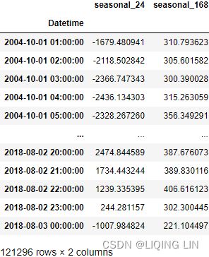
plotly_patterns( results_mstl_win121.seasonal[['seasonal_24']],
                 '2016-01-04', '2016-01-06',
                 '2016-07-04', '2016-07-06',
                 title='Daily pattern in January compared to July',
                 xlabel='Datetime',
                 ylabel='Energy Consumption',
) 
plot_patterns( results_mstl_win121.seasonal[['seasonal_168']],
               '2016-01-04', '2016-01-10',
               '2016-07-04', '2016-07-10',
               title='Weekly pattern in January compared to July',
               xlabel='Datetime',
             )
plotly_patterns( results_mstl_win121.seasonal[['seasonal_168']],
                 '2016-01-04', '2016-01-17',
                 '2016-07-04', '2016-07-17',
                 title='Weekly pattern in January compared to July',
                 xlabel='Datetime',
                 legend_x=0, legend_y=0,
                 nticks=12, tickformat='%d(%A) %H:%M:%S'
               )
To learn more about the MSTL implementation, you can visit the official documentation here: https://www.statsmodels.org/devel/generated/statsmodels.tsa.seasonal.MSTL.html .
Forecasting with multiple seasonal patterns using the Unobserved Components Model (UCM)
In the previous recipe, you were introduced to MSTL to decompose a time series with multiple seasonality. Similarly, the Unobserved Components Model (UCM) is a technique that decomposes a time series (with multiple seasonal patterns), but unlike MSTL, the UCM is also a forecasting model. Initially, the UCM was proposed as an alternative to the ARIMA model and introduced by Harvey in the book Forecasting, structural time series models and the Kalman filter, first published in 1989.
Unlike an ARIMA model, the UCM decomposes a time series process by estimating its components and does not make assumptions regarding stationarity or distribution. Recall, an ARIMA model uses differencing (the d order) to make a time series stationary.
There are situations where making a time series stationary – for example, through differencing – is not achievable. The time series can also contain irregularities and other complexities. This is where the UCM comes in as a more flexible and interpretable model.
The UCM is based on the idea of latent variables or unobserved components of a time series, such as level(ts10_Univariate TS模型_circle mark pAcf_ETS_unpack product_darts_bokeh band interval_ljungbox_AIC_BIC_LIQING LIN的博客-CSDN博客), trend, and seasonality. These can be estimated from the observed variable.
In statsmodels, the UnobservedComponents class decomposes a time series into
- a trend component
 ,
, - a seasonal component
 ,
, - a cyclical component
 , and
, and - an irregular component or error term or disturbance
 .
.
The equation can be generalized as the following:![]()

![]() level equation
level equation![]() slope euation
slope euation
Here,  is the observed variable at time t. You can have multiple seasons as well. The main idea in the UCM is that each component, called state, is modeled in a probabilistic manner, since they are unobserved. The UCM can also contain autoregressive and regression components to capture their effects.
The UCM is a very flexible algorithm that allows for the inclusion of additional models. For example, you use 'level' : 'dtrend' , which specifies the use of a deterministic trend model, adding the following equations:![]()
![]()
You can specify other model to use either by passing the full name, 'level' : 'deterministic trend' , or the abbreviated name, 'dtrend' . The statsmodels library provides an extensive list of models that you can specify – for example, 'local linear deterministic trend' or 'lldtrend' , ' smooth trend' or 'strend' , and 'local linear trend' or 'ltrend' .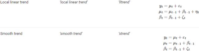
For a complete list of all the available models and the associated equations, you can visit the documentation here: https://www.statsmodels.org/dev/generated/statsmodels.tsa.statespace.structural.UnobservedComponents.html#r0058a7c6fc36-1
Keep in mind that when you provide key-value pairs to the 'freq_seasonal' parameter, each
seasonal component is modeled separately.
In this recipe, you will use the UCM implementation in statsmodels. You will use the same energy dataset loaded in the Technical requirements section. In the Decomposing time series with multiple seasonal patterns using MSTL recipe, you were able to decompose the seasonal pattern into daily, weekly, and yearly components. You will use this knowledge in this recipe:
1. Start by importing the UnobservedComponents class:
from statsmodels.tsa.statespace.structural import UnobservedComponents

plt.rcParams["figure.figsize"] = [14, 4]
2. You will use the UCM model to forecast one month ahead. You will hold out one month to validate the model, and you will split the data to train and test sets accordingly:
# pd.date_range('2004-10-01 01:00:00', '2018-08-03 00:00:00', freq='H')
aep_cp.index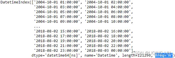
# day = 24                 # 24 hours
# week = day*7             # 168 hours
# month = round(week*4.35) # 731 hours
# year = round(month*12)   # 8772 hours
train = aep_cp.iloc[:-month]
test = aep_cp.iloc[-month:]

train 
ax = train.iloc[-year:].plot( style='k-', alpha=0.45 )
test.plot( ax=ax, style='k' )
plt.show()
The preceding code will display a time series split, one year's worth of hourly energy data from the train set, followed by one month of usage from the test set.
UnobservedComponents
class statsmodels.tsa.statespace.structural.UnobservedComponents(endog, level=False,
   trend=False, seasonal=None, freq_seasonal=None, cycle=False, autoregressive=None,
   exog=None, irregular=False, stochastic_level=False, stochastic_trend=False,
   stochastic_seasonal=True, stochastic_freq_seasonal=None, stochastic_cycle=False,
   damped_cycle=False, cycle_period_bounds=None, mle_regression=True,
   use_exact_diffuse=False, **kwargs)
Univariate unobserved components time series model单变量不可观察成分时间序列模型
These are also known as structural time series models, and decompose a (univariate) time series into trend, seasonal, cyclical, and irregular components.
Parameters: 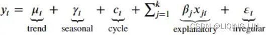
endog array_like
The observed time-series process y
level {bool, str}, optional
Whether or not to include a level component. Default is False. Can also be a string specification of the level / trend component; see Notes for available model specification strings.
trend bool, optional
Whether or not to include a trend component ![]() . Default is False. If True, level must also be True.
. Default is False. If True, level must also be True.
The trend component is a dynamic extension of a regression model that includes an intercept and linear time-trend. It can be written:![]()
![]()


where the level is a generalization of the intercept term水平是截距项的概括 that can dynamically vary across time, and the trend is a generalization of the time-trend such that the slope can dynamically vary across time.
Here  and
and ![]()
For both elements (level and trend), we can consider models in which:
-
The element is included vs excluded (if the trend is included, there must also be a level included).
-
The element is deterministic vs stochastic (i.e. whether or not the variance on the error term(disturbance
) is confined to be zero or not)
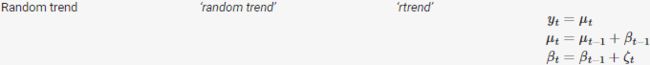
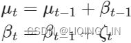
Trends are loosely defined as the natural tendency of the series to increase or decrease or remain constant over a period of time 在没有任何其他影响变量的情况下in absence of any other influencing variable.UCM can model trend in two ways;
- first being the random walk model implying that trend remains roughly constant over the time period of the series, and
- the second being locally linear trend having an upward or downward slope.
seasonal {int, None}, optional
The period of the seasonal component, if any. Default is None.
freq_seasonal {list[dict], None}, optional.
Whether (and how) to model seasonal component(s) with trig. functions是否(以及如何)使用三角函数对季节性成分进行建模. If specified, there is one dictionary for each frequency-domain seasonal component. Each dictionary must have the key, value pair for ‘period’ – integer and may have a key, value pair for ‘harmonics’ – integer. If ‘harmonics’ is not specified in any of the dictionaries, it defaults to the floor of period/2.
cycle bool, optional
Whether or not to include a cycle component. Default is False.
autoregressive {int, None}, optional
The order of the autoregressive component. Default is None.
exog {array_like, None}, optional
Exogenous variables(independent variables).
irregular bool, optional
Whether or not to include an irregular component. Default is False.
stochastic_level bool, optional
Whether or not any level component is stochastic. Default is False.
stochastic_trend bool, optional
Whether or not any trend component is stochastic. Default is False.
stochastic_seasonal bool, optional
Whether or not any seasonal component is stochastic. Default is True.
stochastic_freq_seasonal list[bool], optional
Whether or not each seasonal component(s) is (are) stochastic. Default is True for each component. The list should be of the same length as freq_seasonal.
stochastic_cycle bool, optional
Whether or not any cycle component is stochastic. Default is False.
damped_cycle bool, optional
Whether or not the cycle component is damped周期分量是否阻尼. Default is False.
cycle_period_bounds tuple, optional
A tuple with lower and upper allowed bounds for the period of the cycle. If not provided, the following default bounds are used:
- (1) if no date / time information is provided, the frequency is constrained to be between zero and π, so the period is constrained to be in [0.5, infinity].
- (2) If the date / time information is provided, the default bounds allow the cyclical component to be between 1.5 and 12 years; depending on the frequency of the endogenous variable, this will imply different specific bounds.
mle_regression bool, optional
Whether or not to estimate regression coefficients by maximum likelihood as one of hyperparameters. Default is True. If False, the regression coefficients are estimated by recursive OLS, included in the state vector.
use_exact_diffuse bool, optional
Whether or not to use exact diffuse initialization精确的扩散初始化 for non-stationary states. Default is False (in which case approximate diffuse initialization is used).
The only additional parameters to be estimated via MLE are the variances of any included stochastic components. ![]()
![]()
The level/trend components can be specified using the boolean keyword arguments level, stochastic_level, trend, etc., or all at once as a string argument to level. The following table shows the available model specifications: 


- Time invariant mean
 (
( ,
,  , and
, and are all zero)

- Random walk (initial slope and the slope disturbance covariance are zero)

- Random walk with drift
(the slope disturbance covarianceis zero
(level equation: slope:
 ))
)) 

-
Deterministic time trend
(the level disturbance covariance and the slope disturbance covariance are zero

- Integrated random walk
 (the level disturbance covariance is zero)

Following the fitting of the model, the unobserved level and trend component time series are available in the results class in the level and trend attributes, respectively.
Seasonal (Time-domain)
The seasonal component is modeled as: 
The periodicity (number of seasons) is s, and the defining character is that (without the error term), the seasonal components sum to zero across one complete cycle. The inclusion of an error term allows the seasonal effects to vary over time (if this is not desired,![]() can be set to zero using the stochastic_seasonal=False keyword argument).
can be set to zero using the stochastic_seasonal=False keyword argument).
This component results in one parameter to be selected via maximum likelihood: ![]() , and one parameter to be chosen, the number of seasons s.
, and one parameter to be chosen, the number of seasons s.
Following the fitting of the model, the unobserved seasonal component time series is available in the results class in the seasonal attribute.
Frequency-domain Seasonal
Each frequency-domain seasonal component is modeled as:  where j ranges from 1 to h.
The periodicity (number of “seasons” in a “year”) is s and the number of harmonics is h.(
- As a list of s numbers that sum to zero
- As a sum of [s/2] deterministic, undamped cycles, called harmonics, of periods s, s/2, s/3,
…
Here [s/2] = s/2 if s is even and [s/2] = (s-1)/2 if s is odd.
Example:
For s = 12, the seasonal pattern can always be written as a sum of six cycles with periods 12, 6, 4, 3, 2.4, and 2.
s = 12 for monthly data, s = 4 for quarterly data, and s = 2 for bi-annual data.
) Note that h is configurable to be less than s/2, but s/2 harmonics is sufficient to fully model all seasonal variations of periodicity s. Like the time domain seasonal term (cf. Seasonal section, above), the inclusion of the error terms allows for the seasonal effects to vary over time. The argument stochastic_freq_seasonal can be used to set one or more of the seasonal components of this type to be non-random, meaning they will not vary over time.
This component results in one parameter to be fitted using maximum likelihood: ![]() , and up to two parameters to be chosen, the number of seasons s and optionally the number of harmonics h, with 1≤h≤⌊s/2⌋.
, and up to two parameters to be chosen, the number of seasons s and optionally the number of harmonics h, with 1≤h≤⌊s/2⌋.
After fitting the model, each unobserved seasonal component modeled in the frequency domain is available in the results class in the freq_seasonal attribute.
Cycle
The cyclical component is intended to capture cyclical effects at time frames much longer than captured by the seasonal component (In general, the average length of cycles is longer than the length of a seasonal pattern, and the magnitudes of cycles tend to be more variable than the magnitudes of seasonal patterns.ts9_annot_arrow_hvplot PyViz interacti_bokeh_STL_seasonal_decomp_HodrickP_KPSS_F-stati_Box-Cox_Ljung_LIQING LIN的博客-CSDN博客). For example, in economics the cyclical term is often intended to capture the business cycle, and is then expected to have a period between “1.5 and 12 years” (see Durbin and Koopman).

The parameter ![]() (the frequency of the cycle) is an additional parameter to be estimated by MLE.
(the frequency of the cycle) is an additional parameter to be estimated by MLE.
If the cyclical effect is stochastic (stochastic_cycle=True), then there is another parameter to estimate (the variance of the error term - note that both of the error terms here share the same variance, but are assumed to have independent draws).
If the cycle is damped (damped_cycle=True), then there is a third parameter to estimate, ![]() .
.
In order to achieve cycles with the appropriate frequencies, bounds are imposed on the parameter ![]() in estimation. These can be controlled via the keyword argument cycle_period_bounds, which, if specified, must be a tuple of bounds on the period (lower, upper). The bounds on the frequency are then calculated from those bounds.
in estimation. These can be controlled via the keyword argument cycle_period_bounds, which, if specified, must be a tuple of bounds on the period (lower, upper). The bounds on the frequency are then calculated from those bounds.
The default bounds, if none are provided, are selected in the following way:
-
If no date / time information is provided, the frequency is constrained to be between zero and π, so the period is constrained to be in [0.5,∞].
-
If the date / time information is provided, the default bounds allow the cyclical component to be between 1.5 and 12 years; depending on the frequency of the endogenous variable(dependent variables, Endogenous variables are influenced by other variables within the systemts12_2Multi-step Forecast_sktime_KNeighbors_WindowSplitter_ForecastingGridSearchCV_exog_EnsembleFore_LIQING LIN的博客-CSDN博客), this will imply different specific bounds.
Following the fitting of the model, the unobserved cyclical component time series is available in the results class in the cycle attribute.
Irregular
The irregular components are independent and identically distributed (iid): ![]()
Autoregressive Irregular
An autoregressive component (often used as a replacement for the white noise irregular term) can be specified as: 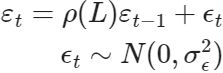
In this case, the AR order is specified via the autoregressive keyword, and the autoregressive coefficients are estimated.
Following the fitting of the model, the unobserved autoregressive component time series is available in the results class in the autoregressive attribute.
Regression effects
Exogenous regressors can be pass to the exog argument. The regression coefficients will be estimated by maximum likelihood unless mle_regression=False, in which case the regression coefficients will be included in the state vector where they are essentially estimated via recursive OLS.
If the regression_coefficients are included in the state vector, the recursive estimates are available in the results class in the regression_coefficients attribute.https://medium.com/analytics-vidhya/tsa-ucm-python-5fde69d42e28
4. UnobservedComponents takes several parameters. Of interest is freq_seasonal, which takes a dictionary for each frequency-domain seasonal component – for example, daily, weekly, and annually. You will
- pass a list of key-value pairs for each period.
- Optionally, within each dictionary, you can also pass a key-value pair for harmonics.
- If no harmonic values are passed, then the default would be the np.floor(period/2) :
params = { 'level':'dtrend',
           'irregular':True,
           'freq_seasonal':[{'period': day, 'harmonics':2},
                            {'period': week, 'harmonics':2},
                            {'period': year, 'harmonics':2}
                           ],
           'stochastic_freq_seasonal':[False, False, False]
         }
model_uc = UnobservedComponents( train, **params )
By default, the fit method uses the lbfgs solver.
results_uc = model_uc.fit()available .fit() methods. Default is lbfgs
    'newton' for Newton-Raphson
    'nm' for Nelder-Mead
    'bfgs' for Broyden-Fletcher-Goldfarb-Shanno (BFGS)
    'lbfgs' for limited-memory BFGS with optional box constraints
    'powell' for modified Powell's method
    'cg' for conjugate gradient
    'ncg' for Newton-conjugate gradient
    'basinhopping' for global basin-hopping solver
5. Once training is complete, you can view the model's summary using the summary method:
results_uc.summary() The results objects is of type UnobservedComponentsResultsWrapper, which gives access to several properties and methods, such as plot_components and plot_diagnostics, to name a few.
results_uc![]()
6. plot_diagnostics is used to diagnose the model's overall performance against the residuals:
fig = results_uc.plot_diagnostics( figsize=(12, 6) )
fig.tight_layout()
Figure 15.3 – Residual diagnostics plots
7. You can plot the components, which will produce six subplots using the smoothed results –
- predicted versus observed,
- the level component,
- the trend component,
- seasonal(24),
- seasonal(168), and
- seasonal(8772).
results_uc.freq_seasonal
The plots for freq_seasonal are too condensed (given the number of observations) to visibly see any pattern for the daily and weekly seasonal components. Instead, you will plot each component individually by slicing the data. For now, use plot_components , but disable the freq_seasonal output, as shown in the following:
fig = results_uc.plot_components( figsize=(10,10),
                                  freq_seasonal=False,
                                  which='smoothed'
                                )
#fig.tight_layout()
Figure 15.4 – Plot for three components from the UCM model
8. You can access the data behind each component from the results object. For example, you can access freq_seasonal , which should contain a list of three dictionaries, one for each seasonal period, daily, weekly, and yearly, based on what you provided in the key-value pair when you initialized the model (see Step 4). Each dictionary contains six outputs or keys, as shown in the following:
results_uc.freq_seasonal
results_uc.freq_seasonal[0].keys()![]()
You will plot using the smoothed results for each period, starting with daily.
9. Plot the daily seasonal component. For easier interpretation, slice the data to show 24 hours (1 day): ts12_2Multi-step Forecast_sktime_KNeighbors_WindowSplitter_ForecastingGridSearchCV_exog_EnsembleFore_LIQING LIN的博客-CSDN博客
We have used the following character strings to format the date:
%b: Returns the first three characters of the month name. In our example, it returned "Sep".%d: Returns day of the month, from 1 to 31. In our example, it returned "15".%Y: Returns the year in four-digit format. In our example, it returned "2022".%H: Returns the hour. In our example, it returned "00".%M: Returns the minute, from 00 to 59. In our example, it returned "00".%S: Returns the second, from 00 to 59. In our example, it returned "00".
Other than the character strings given above, the strftime method takes several other directives for formatting date values:How to Format Dates in Python
%a: Returns the first three characters of the weekday, e.g. Wed.%A: Returns the full name of the weekday, e.g. Wednesday.%B: Returns the full name of the month, e.g. September.%w: Returns the weekday as a number, from 0 to 6, with Sunday being 0.%m: Returns the month as a number, from 01 to 12.%p: Returns AM/PM for time.%y: Returns the year in two-digit format, that is, without the century. For example, "18" instead of "2018".%f: Returns microsecond from 000000 to 999999.%Z: Returns the timezone.%z: Returns UTC offset.%j: Returns the number of the day in the year, from 001 to 366.%W: Returns the week number of the year, from 00 to 53, with Monday being counted as the first day of the week.%U: Returns the week number of the year, from 00 to 53, with Sunday counted as the first day of each week.%c: Returns the local date and time version.%x: Returns the local version of date.%X: Returns the local version of time.
daily = pd.DataFrame( results_uc.freq_seasonal[0]['smoothed'],
                      index=train.index,
                      columns=['y']
                    ) # day = 24 hours
# %I : Hour (00 to 12)
# %M : Minute (00 to 59)
# %S : Second (00 to 59)
# %p : AM/PM
daily['hour_of_day'] = daily.index.strftime( date_format = '%I:%M:%S %p' )
daily.iloc[:day].plot( y='y', x='hour_of_day', title='Daily Seasonality', figsize=(12,4) )
plt.show()
The preceding code should show a plot representing 24 hours (zoomed in) to focus on the daily pattern. The x-axis ticker labels are formatted to display the time (and AM/PM):
Figure 15.5 – Plotting the daily seasonal component
Note that the spike in energy consumption starts around 11:00 AM, peaking at around 9:00 PM, and then declines during the sleeping time until the following day. We had a similar observation in the previous recipe using MSTL .
from datetime import datetime
def plotly_pattern(df,
title, xlabel, ylabel=None,
legend_x=0, legend_y=1,
tickformat='%I:%M:%S %p'
):
layout=go.Layout(width=1000, height=500,
xaxis=dict(title=xlabel, color='black', tickangle=-30),
yaxis=dict(title=ylabel, color='black'),
title=dict(text=title,
x=0.5, y=0.9
),
)
fig = go.Figure(layout=layout)
# https://plotly.com/python/marker-style/#custom-marker-symbols
# circle-open-dot
# https://support.sisense.com/kb/en/article/changing-line-styling-plotly-python-and-r
fig.add_trace( go.Scatter( name='y',
mode ='lines', #marker_symbol='circle',
line=dict(shape = 'linear', color = 'blue',#'rgb(100, 10, 100)',
width = 2, #dash = 'dashdot'
),
x=df.index,#df[df.columns[-1]].values,
y=df['y'].values,
hovertemplate = 'energy: %{y:.2f}
daily_filtered = pd.DataFrame( results_uc.freq_seasonal[0]['filtered'],
                               index=train.index,
                               columns=['y']
                             ) # day = 24 hours
plotly_pattern(daily_filtered[:2*day], title='Daily Seasonality(filtered)',
               xlabel='hour_of_day', ylabel='energy consumption',
               legend_x=0, legend_y=0,
)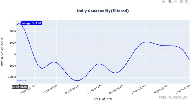 10. Plot the weekly component. Similarly, slice the data (zoom in) to show only one week–ideally, Sunday to Sunday – as shown in the following:
weekly = pd.DataFrame( results_uc.freq_seasonal[1]['smoothed'],
                       index=train.index, columns=['y']
                     )
weekly['day_name'] = weekly.index.strftime(date_format='%A')
weekly.loc['2004-10-03': '2004-10-10'].plot( y='y',
                                             x='day_name',
                                             title='Week Seasonality',
                                             figsize=(12,4)
                                           )
plt.show()
The preceding code should produce a plot showing a whole week to observe the weekly seasonal component. The x-axis ticker labels will display the day's name to make it easier to compare weekends and weekdays:
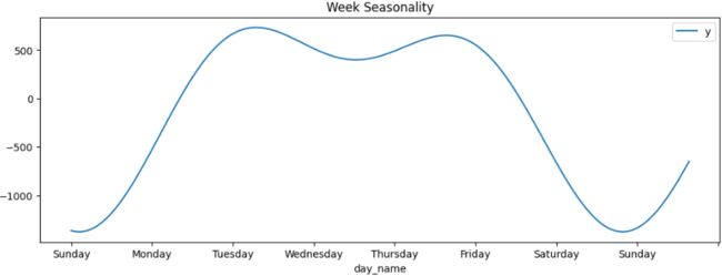
Figure 15.6 – Plotting the weekly seasonal component
Notice the spikes during the weekdays (Monday to Friday), which later dip during the weekend. We had a similar observation in the previous recipe using MSTL.
plotly_pattern(weekly.loc['2004-10-03': '2004-10-17'],
               title='Week Seasonality',
               xlabel='day_name', ylabel='energy consumption',
               tickformat='%A(%Y-%m-%d)'
) 
weekly_filtered = pd.DataFrame( results_uc.freq_seasonal[1]['filtered'],
                                index=train.index, columns=['y']
                              )
plotly_pattern(weekly_filtered.loc['2004-10-03': '2004-10-17'],
               title='Week Seasonality(filtered)',
               xlabel='day_name', ylabel='energy consumption',
               tickformat='%A(%Y-%m-%d)'
) 11. Plot the annual seasonal component. Similarly, slice the data to show a full year (January to December):
annual = pd.DataFrame( results_uc.freq_seasonal[2]['smoothed'],
                       index=train.index,
                       columns=['y']
                     )
annual['month'] = annual.index.strftime(date_format='%B')
ax = annual.loc['2005'].plot(y='y', x='month',
                             title='Annual Seasonality',
                             figsize=(12,4)
                            )
The preceding code should produce a plot 1 full year from the yearly seasonal component. The x-axis ticker labels will display the month name:

Figure 15.7 – Plotting the yearly seasonal component
Notice the spike in January and another spike from July to August.
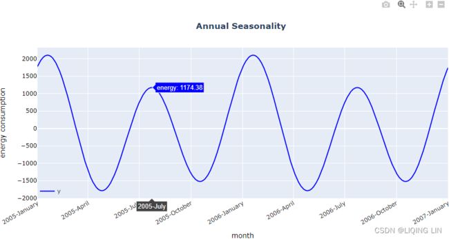
plotly_pattern(annual.loc['2005':'2006'],
               title='Annual Seasonality',
               xlabel='month', ylabel='energy consumption',
               tickformat='%Y-%B',
               legend_x=0, legend_y=0,
              )
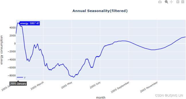
annual_filtered = pd.DataFrame( results_uc.freq_seasonal[2]['filtered'],
                                index=train.index,
                                columns=['y']
                              )
plotly_pattern(annual_filtered.loc['2005'],
               title='Annual Seasonality(filtered)',
               xlabel='month', ylabel='energy consumption',
               tickformat='%Y-%B',
               legend_x=0, legend_y=0,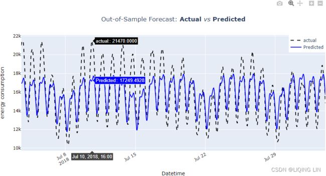
)  12. Finally, use the model to make a prediction and compare it against the out-of-sample set (test data):
test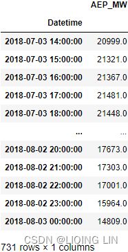
prediction_uc = results_uc.predict( start=test.index.min(),
                                    end=test.index.max()
                                  )
test.plot( style='k--', alpha=0.5, figsize=(12,4) )
prediction_uc.plot( style='b' )
plt.legend(['Actual', 'Predicted'])
plt.title('Out-of-Sample Forecast: Actual vs Predicted')
plt.show() Figure 15.8 – Actual versus predicted using the UCM
import plotly.graph_objects as go
from plotly.subplots import make_subplots
def plotly_forecast( model, test, title,
xlabel='Datetime', ylabel='energy consumption',
legend_x=0.88, legend_y=1
):
layout=go.Layout(width=1000, height=500,
xaxis=dict(title=xlabel, color='black', tickangle=-30),
yaxis=dict(title=ylabel, color='black'),
title=dict(text=title,
x=0.5, y=0.9
),
)
fig = go.Figure(layout=layout)
precision=4
fig.add_trace( go.Scatter( name='actual',
mode ='lines',
line=dict(shape = 'linear', color = 'black', #'rgb(100, 10, 100)',
width = 2, dash = 'dash'
),
x=test.index,
y=test['AEP_MW'].values,
hovertemplate='
'.join([ #'Epoch: %{x}/500',
"actual:" + f": %{{y:.{precision}f}}",
'
'.join([ #'Epoch: %{x}/500',
"Predicted:" + f": %{{y:.{precision}f}}",
'
13. Calculate the RMSE and RMSPE(Root Mean Square Percentage Error) using the functions imported from statsmodels earlier in the Technical requirements section. You will use the scores to compare with other methods:
Mean Square Percentage Error(MSPE): ![]()
Root Mean Square Percentage Error(RMSPE): ![]()
from statsmodels.tools.eval_measures import rmse, rmspe

rmspe( test['AEP_MW'], prediction_uc ) 
rmse( test['AEP_MW'], prediction_uc ) ![]()
Rerun the same UCM model, but this time, reduce the harmonics to one (1):
params = { 'level':'dtrend',
           'irregular':True,
           'freq_seasonal':[{'period': day, 'harmonics':1},
                            {'period': week, 'harmonics':1},
                            {'period': year, 'harmonics':1}
                           ],
           'stochastic_freq_seasonal':[False, False, False]
         }
model_uc_h1 = UnobservedComponents( train, **params )
results_uc_h1 = model_uc_h1.fit()
results_uc_h1.summary()
If you run the component plots, you will notice that all the plots are overly smoothed. This is even more obvious if you plot the predicted values against the test data.
fig = results_uc_h1.plot_diagnostics( figsize=(12, 6) )
fig.tight_layout()
fig = results_uc_h1.plot_components( figsize=(10,10),
                                     freq_seasonal=False,
                                     which='smoothed'
                                   )
#fig.tight_layout()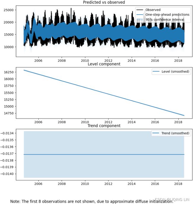
daily = pd.DataFrame( results_uc.freq_seasonal[0]['smoothed'],
                               index=train.index,
                               columns=['y']
                             )
daily['hour_of_day'] = daily.index.strftime(date_format = '%I:%M:%S %p')

daily_uc_h1 = pd.DataFrame( results_uc_h1.freq_seasonal[0]['smoothed'],
                            index=train.index,
                            columns=['y']
                          )
daily_uc_h1['hour_of_day'] = daily_uc_h1.index.strftime(date_format = '%I:%M:%S %p')
# %I : Hour (00 to 12)
# %M : Minute (00 to 59)
# %S : Second (00 to 59)
# %p : AM/PM
daily_uc_h1['hour_of_day'] = daily_uc_h1.index.strftime( date_format = '%I:%M:%S %p' )
ax=daily_uc_h1.iloc[:day].plot( y='y', x='hour_of_day',
                                title='Daily Seasonality', figsize=(12,4)
                              )
daily.iloc[:day].plot( y='y', x='hour_of_day',
                       ax=ax
                     )
ax.legend(['y_1_harmonic(s)', 'y_2_harmonic(s)'])
plt.show()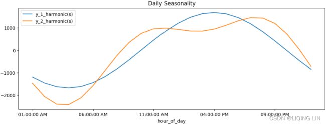
weekly_uc_h1 = pd.DataFrame( results_uc_h1.freq_seasonal[1]['smoothed'],
                             index=train.index, columns=['y']
                           )
weekly_uc_h1['day_name'] = weekly_uc_h1.index.strftime(date_format='%A')

ax=weekly_uc_h1.loc['2004-10-03': '2004-10-10'].plot( y='y',
                                                      x='day_name',
                                                      title='Week Seasonality',
                                                      figsize=(12,4)
                                                    )

weekly.loc['2004-10-03': '2004-10-10'].plot( y='y',
                                             x='day_name',
                                             ax=ax
                                           )
ax.legend(['y_1_harmonic(s)', 'y_2_harmonic(s)'])
plt.show()
annual_uc_h1 = pd.DataFrame( results_uc_h1.freq_seasonal[2]['smoothed'],
                             index=train.index,
                             columns=['y']
                           )
annual_uc_h1['month'] = annual_uc_h1.index.strftime(date_format='%B')
ax = annual_uc_h1.loc['2005'].plot(y='y', x='month',
                             title='Annual Seasonality',
                             figsize=(12,4)
                            )
annual.loc['2005'].plot(y='y', x='month',
                        ax=ax
                       )
ax.legend(['y_1_harmonic(s)', 'y_2_harmonic(s)'])
plt.show()
prediction_uc_h1 = results_uc_h1.predict( start=test.index.min(),
                                          end=test.index.max()
                                        )
test.plot( style='k--', alpha=0.5, figsize=(12,4) )
prediction_uc_h1.plot( style='b' )
prediction_uc.plot( style='g' )
plt.legend(['Actual', 'Predicted_1_harmonic(s)','Predicted_2_harmonic(s)'])
plt.title('Out-of-Sample Forecast: Actual vs Predicted(1h) vs Predicted(2h)')
plt.show() Figure 15.9 – The UCM forecast versus the actual with lower harmonic values and with higher harmonic values
Calculate RMSE and RMSPE and compare against the first UMC model:
print( rmspe(test['AEP_MW'], prediction_uc_h1) )
print( rmspe(test['AEP_MW'], prediction_uc) ) ![]()
print( rmse(test['AEP_MW'], prediction_uc_h1) )
print( rmse(test['AEP_MW'], prediction_uc) ) ![]()
This model overly generalizes(underfitting), producing overly smoothed results, making it perform much worse than the first model.
To learn more about the UCM implementation in statsmodels, you can visit the offcial documentation here: https://www.statsmodels.org/dev/generated/statsmodels.tsa.statespace.structural.UnobservedComponents.html
Forecasting time series with multiple seasonal patterns using Prophet
You were introduced to Prophet in ts11_pmdarima_edgecolor_bokeh plotly_Prophet_Fourier_VAR_endog exog_Granger causality_IRF_Garch vola_LIQING LIN的博客-CSDN博客, Additional Statistical Modeling Techniques for Time Series, under the Forecasting time series data using Facebook Prophet recipe, using the milk production dataset. The milk production dataset is a monthly dataset with a trend and one seasonal pattern.
The goal of this recipe is to show how you can use Prophet to solve a more complex dataset with multiple seasonal patterns. Preparing time series data for supervised learning is an important step, as shown in ts12_Multi-step Forecast_sktime_bold_Linear Regress_sMAPE MASE_warn_plotly acf vlines_season_summary_LIQING LIN的博客-CSDN博客ts12_2Multi-step Forecast_sktime_KNeighbors_WindowSplitter_ForecastingGridSearchCV_exog_EnsembleFore_LIQING LIN的博客-CSDN博客, Forecasting Using Supervised Machine Learning, and ts13_install tf env_RNN_Bidirectional LSTM_GRU_Minimal gated_TimeDistributed_Time Series Forecasting_LIQING LIN的博客-CSDN博客, Deep Learning for Time Series Forecasting. Similarly, the feature engineering technique for creating additional features is an important topic when training and improving machine learning and deep learning models. One benefit of using algorithms such as the UCM (introduced in the previous recipe) or Prophet is that they require little to no data preparation, can work with noisy data, and are easy to interpret. Another advantage is their ability to decompose a time series into its components (trend and multiple seasonal components).
In this recipe, you will continue using the same energy consumption dataset (the df DataFrame) and perform a similar split for the train and test sets. If you recall, in Prophet, you had to reset the index and rename the index and the observed column as ds and y respectively:
# https://github.com/facebook/prophet/blob/main/python/prophet/forecaster.py
    def fit(self, df, **kwargs):
        """Fit the Prophet model.
        This sets self.params to contain the fitted model parameters. It is a
        dictionary parameter names as keys and the following items:
            k (Mx1 array): M posterior samples of the initial slope.
            m (Mx1 array): The initial intercept.
            delta (MxN array): The slope change at each of N changepoints.
            beta (MxK matrix): Coefficients for K seasonality features.
            sigma_obs (Mx1 array): Noise level.
        Note that M=1 if MAP estimation.
        Parameters
        ----------
        df: pd.DataFrame containing the history. Must have columns ds (date
            type) and y, the time series. If self.growth is 'logistic', then
            df must also have a column cap that specifies the capacity at
            each ds.
        kwargs: Additional arguments passed to the optimizing or sampling
            functions in Stan.
        Returns
        -------
        The fitted Prophet object.
        """
        if self.history is not None:
            raise Exception('Prophet object can only be fit once. '
                            'Instantiate a new object.')
        if ('ds' not in df) or ('y' not in df):
            raise ValueError(
                'Dataframe must have columns "ds" and "y" with the dates and '
                'values respectively.'
            )
        history = df[df['y'].notnull()].copy()
        if history.shape[0] < 2:
            raise ValueError('Dataframe has less than 2 non-NaN rows.')
        self.history_dates = pd.to_datetime(pd.Series(df['ds'].unique(), name='ds')).sort_values()

        history = self.setup_dataframe(history, initialize_scales=True)
        self.history = history
        self.set_auto_seasonalities()
        seasonal_features, prior_scales, component_cols, modes = (
            self.make_all_seasonality_features(history))
        self.train_component_cols = component_cols
        self.component_modes = modes
        self.fit_kwargs = deepcopy(kwargs)

        self.set_changepoints()

        trend_indicator = {'linear': 0, 'logistic': 1, 'flat': 2}

        dat = {
            'T': history.shape[0],
            'K': seasonal_features.shape[1],
            'S': len(self.changepoints_t),
            'y': history['y_scaled'],
            't': history['t'],
            't_change': self.changepoints_t,
            'X': seasonal_features,
            'sigmas': prior_scales,
            'tau': self.changepoint_prior_scale,
            'trend_indicator': trend_indicator[self.growth],
            's_a': component_cols['additive_terms'],
            's_m': component_cols['multiplicative_terms'],
        }

        if self.growth == 'linear':
            dat['cap'] = np.zeros(self.history.shape[0])
            kinit = self.linear_growth_init(history)
        elif self.growth == 'flat':
            dat['cap'] = np.zeros(self.history.shape[0])
            kinit = self.flat_growth_init(history)
        else:
            dat['cap'] = history['cap_scaled']
            kinit = self.logistic_growth_init(history)

        stan_init = {
            'k': kinit[0],
            'm': kinit[1],
            'delta': np.zeros(len(self.changepoints_t)),
            'beta': np.zeros(seasonal_features.shape[1]),
            'sigma_obs': 1,
        }

        if history['y'].min() == history['y'].max() and \
                (self.growth == 'linear' or self.growth == 'flat'):
            self.params = stan_init
            self.params['sigma_obs'] = 1e-9
            for par in self.params:
                self.params[par] = np.array([self.params[par]])
        elif self.mcmc_samples > 0:
            self.params = self.stan_backend.sampling(stan_init, dat, self.mcmc_samples, **kwargs)
        else:
            self.params = self.stan_backend.fit(stan_init, dat, **kwargs)

        self.stan_fit = self.stan_backend.stan_fit
        # If no changepoints were requested, replace delta with 0s
        if len(self.changepoints) == 0:
            # Fold delta into the base rate k
            self.params['k'] = (
                self.params['k'] + self.params['delta'].reshape(-1)
            )
            self.params['delta'] = (np.zeros(self.params['delta'].shape)
                                      .reshape((-1, 1)))

        return
1. Start by importing the Prophet library:
from prophet import Prophet
from prophet.plot import add_changepoints_to_plot
2. You already loaded the dataset into a pandas DataFrame (as df ) in the Technical requirements section.
import pandas as pd

# from pathlib import Path

# folder = Path('./archive/')
# aep_file = folder.joinpath('AEP_hourly.csv')
# aep = pd.read_csv( aep_file,# American Electric Power
#                    index_col='Datetime',
#                    parse_dates=True
#                  )

base='https://raw.githubusercontent.com/PacktPublishing/Time-Series-Analysis-with-Python-Cookbook/main/datasets/Ch15/'

aep = pd.read_csv( base+'AEP_hourly.csv',# American Electric Power
                   index_col='Datetime',
                   parse_dates=True
                 )
aep_cp = aep.copy(deep=True)        #####
aep_cp.sort_index(inplace=True)     ##### sort the index
aep_cp = aep_cp.resample('H').max() ##### resample
#Forward filling: ffill or pad ,
#uses the last value before the missing spot(s) and fills the gaps forward
aep_cp.ffill(inplace=True)
aep_cp.columns = ['y']              ##### rename
aep_cp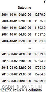 You will need to reset the index and rename the columns to use in Prophet. Start by making a copy of the original DataFrame, since you will be using it for other recipes:
energy = aep_cp.copy( deep=True )
energy.reset_index( inplace=True )
energy.columns = ['ds','y']
energy  then
then
3. Split the data into train and test sets using the same split from the previous recipe:
day = 24                 # 24 hours
week = day*7             # 168 hours
month = round(week*4.35) # 731 hours
year = round(month*12)   # 8772 hours

train = energy.iloc[:-month]
test = energy.iloc[-month:]
train 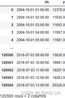
![]()
4. Fit the model using all default options and have Prophet automatically detect the seasonal components. If you recall, the train DataFrame is already set to the H frequency:
https://github.com/facebook/prophet/blob/main/python/prophet/forecaster.py

    def __init__(
            self,
            growth='linear',
            changepoints=None,
            n_changepoints=25,
            changepoint_range=0.8,
            yearly_seasonality='auto',
            weekly_seasonality='auto',
            daily_seasonality='auto',
            holidays=None,
            seasonality_mode='additive',
            seasonality_prior_scale=10.0,
            holidays_prior_scale=10.0,
            changepoint_prior_scale=0.05,
            mcmc_samples=0,
            interval_width=0.80,
            uncertainty_samples=1000,
            stan_backend=None
    ):
Prophet automated many aspects of building and optimizing the model because yearly_seasonality , weekly_seasonality , and daily_seasonality parameters were set to auto by default, allowing Prophet to determine which ones to turn on or of based on the data.
model = Prophet().fit(train)
In Chapter 11, Additional Statistical Modeling Techniques for Time Series, when you fit the model on the milk data, you got these two messages:
INFO: prophet: Disabling weekly seasonality. Run prophet
with weekly_seasonality=True to override this.
INFO: prophet: Disabling daily seasonality. Run prophet
with daily_seasonality=True to override this.
The messages indicate that Prophet did not detect weekly or daily seasonal patterns and turned them off. But now, using the energy consumption data, you should not see any message. This indicates Prophet has already identified all three – the daily, weekly, and yearly seasonal patterns.
5. Use the make_future_dataframe method to extend the train DataFrame forward for a specific number of periods and at a specified frequency. In this case, it will be the number of test observations:
n = len(test)
future = model.make_future_dataframe(n, freq='H',
                                     include_history=True #default
                                    )
future The frequency is indicated as hourly with freq='H' .
6. Use the predict method, which takes the future DataFrame for making predictions. If you recall, Prophet will make in-sample predictions to cover the entire period from the train set and then extend to future predictions (this will be compared to the out-of-sample test dataset):
forecast = model.predict(future)
forecast

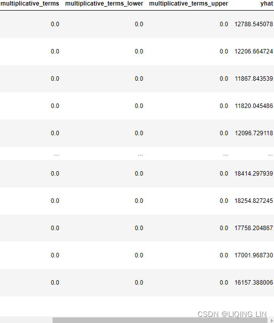
7. Inspect the components using the plot_components method:
import matplotlib.pyplot as plt

model.plot_components(forecast)
plt.show()
The preceding code should produce four subplots, representing the trend, weekly, yearly, and daily seasonal trends. The following only shows the seasonal components: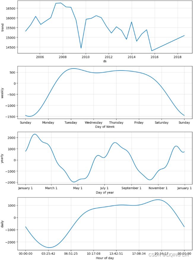 Figure 15.10 – Time series seasonal components automatically detected by Prophet
import matplotlib.dates as mdates
fig, axes = plt.subplots( 4,1, figsize=(12, 12) )

axes[0].plot( forecast['ds'], forecast['trend'] )
axes[0].set_xlabel('ds')
axes[0].set_ylabel('trend')

week_select=forecast[('2004-10-03' <=forecast['ds']) & (forecast['ds']<='2004-10-10')]
axes[1].plot( week_select['ds'], week_select['weekly'] )
axes[1].xaxis.set_major_formatter( mdates.DateFormatter('%A') )
axes[1].set_xlabel('Day of week')
axes[1].set_ylabel('weekly')

year_select=forecast[('2005'<=forecast['ds']) & (forecast['ds']<'2006') ]
#year_select.set_index('ds', inplace=True)
#year_select['month'] = year_select.index.strftime(date_format='%B %-d')
axes[2].plot( year_select['ds'], year_select['yearly'] )
axes[2].xaxis.set_major_formatter( mdates.DateFormatter('%B %d') )
axes[2].set_xlabel('Day of year')
axes[2].set_ylabel('yearly')

axes[3].plot( forecast[:day]['ds'], forecast[:day]['daily'])
axes[3].xaxis.set_major_formatter( mdates.DateFormatter('%H:%M:%S') )
axes[3].set_xlabel('Hour of day')
axes[3].set_ylabel('daily')

plt.subplots_adjust(hspace = 0.4)
plt.show()
Compare the seasonal components from Prophet in Figure 15.10 with those obtained from the UMC (Figure 15.5, Figure 15.6, and Figure 15.7). Overall, the daily and weekly components in Figure 15.10 look similar to those from the UMC. The difference is in the yearly component; there are more wiggles in Figure 15.10(prophet) when compared to a smoother plot in Figure 15.7(UMC).
8. The forecast DataFrame contains the predicted values for in-sample and out-of-sample under the yhat column. Slice the forecast DataFrame to show only the out-of-sample predictions and compare them with the test set.
prediction = forecast.iloc[ test.index[0]: ].set_index('ds')['yhat']
prediction  vs
vs
You can now use this sliced DataFrames for plotting, similar to the plot created in Figure 15.8:
import plotly.graph_objects as go
from plotly.subplots import make_subplots
def plotly_forecast( prediction, test, title,
xlabel='Datetime', ylabel='energy consumption',
legend_x=0.88, legend_y=1
):
layout=go.Layout(width=1000, height=500,
xaxis=dict(title=xlabel, color='black', tickangle=-30),
yaxis=dict(title=ylabel, color='black'),
title=dict(text=title,
x=0.5, y=0.9
),
)
fig = go.Figure(layout=layout)
precision=4
fig.add_trace( go.Scatter( name='actual',
mode ='lines',
line=dict(shape = 'linear', color = 'black', #'rgb(100, 10, 100)',
width = 2, dash = 'dash'
),
x=test['ds'].values,
y=test['y'].values,
hovertemplate='
'.join([ #'Epoch: %{x}/500',
"actual:" + f": %{{y:.{precision}f}}",
'
'.join([ #'Epoch: %{x}/500',
"Predicted:" + f": %{{y:.{precision}f}}",
' The preceding code should produce a time series plot showing the actual (test) data against the predicted values from Prophet: Figure 15.11 – Actual versus Predicted with Prophet
9. Calculate the RMSE and RMSPE values:
from statsmodels.tools.eval_measures import rmse, rmspe

rmspe( test['y'], prediction.values )![]()
rmse( test['y'], prediction.values ) 
Based on RMSE and RMSPE, the UMC model in Figure 15.8 performed better than the Prophet model. The UMC scores were and ![]() for RMSE and RMSPE respectively.
for RMSE and RMSPE respectively.
So far, you have used Prophet on time series with single seasonality(ts11_pmdarima_edgecolor_bokeh plotly_Prophet_Fourier_VAR_endog exog_Granger causality_IRF_Garch vola_LIQING LIN的博客-CSDN博客) and now again on a time series with multiple seasonality. The process for training a model and making predictions is the same, making Prophet a very appealing option due to its consistent framework.
One of the nice things about Prophet is that the algorithm uses changepoint detection, and you can display the significant changepoints using the add_changepoints_to_plot function. If you recall from Chapter 11, Additional Statistical Modeling Techniques for Time Series, Prophet initially starts with 25 changepoints, using 80% of the training data:
fig = model.plot( forecast, ylabel='Energy Consumption' )
add_changepoints_to_plot( fig.gca(), model, forecast, threshold=0.01 )
plt.show() Figure 15.12 – Using Prophet to display the significant changepoints and the forecast
from prophet.plot import plot_plotly, plot_components_plotly, add_changepoints_to_plot

# https://github.com/facebook/prophet/blob/v0.5/python/fbprophet/plot.py#L42
fig=plot_plotly( model, forecast,
                 ylabel='Energy Consumption',
                 trend=True,
                 changepoints=True,
                 figsize=(800,800)
               )
fig.show()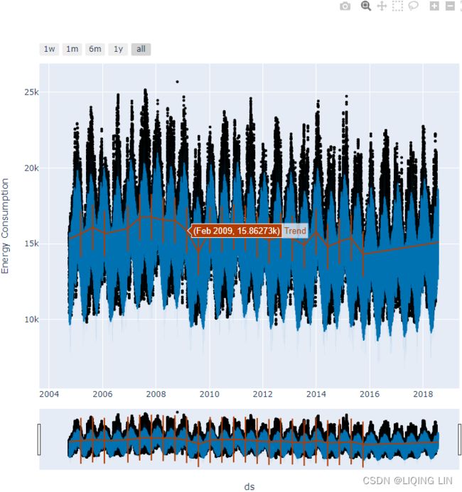 In the add_changepoints_to_plot function, the threshold parameter is set to 0.01 (default), and increasing the value will reduce the number of changepoints displayed. Compare the trend line in Figure 15.12 to the trend component obtained from step 7 (using plot_components)
 Figure 15.13 – The trend component from Prophet
This aligns with how the piece-wise regression was determined based on the detected changepoints. The inflection points in the trend are based on those changepoints趋势中的拐点基于这些变化点.
Prophet supports both Python and R. For more information on the Python API, visit the documentation here: https://facebook.github.io/prophet/docs/quick_start.html#python-api .
Forecasting time series with multiple seasonal patterns using NeuralProphet
NeuralProphet was inspired by the Prophet library and Autoregressive Neural Network (AR-Net) to bring a new implementation, leveraging deep neural networks to provide a more scalable solution.
Prophet was built on top of PyStan, a Bayesian inference library, and is one of the main dependencies when installing Prophet. Conversely, NeuralProphet is based on PyTorch and is as used as the deep learning framework. This allows NeuralProphet to scale to larger datasets and generally provides better accuracy than Prophet. Like Prophet's method, NeuralProphet performs hyperparameter tuning and fully automates many aspects of time series forecasting.
In this recipe, you will compare the results using NeuralProphet against Prophet.
The following instructions will show how to create a virtual environment using conda . You can call the environment any name you like – in the following example, we will name our environment neuralprophet
conda create -n neuralprophet python=3.9 -y
conda activate neuralprophet

pip install "neuralprophet[live]" 
To make the new neuralprophet environment visible within Jupyter, you can run the following code:
pip install ipykernel
python -m ipykernel install --user --name neuralprophet --display-name "NeuralProphet"![]()
pip install jupyter notebook
you can copy a shortcut from other jupyter notebook then rename it to
'Jupyter Notebook (neuralprophet)':
C:\ProgramData\Microsoft\Windows\Start Menu\Programs\Anaconda3 (64-bit)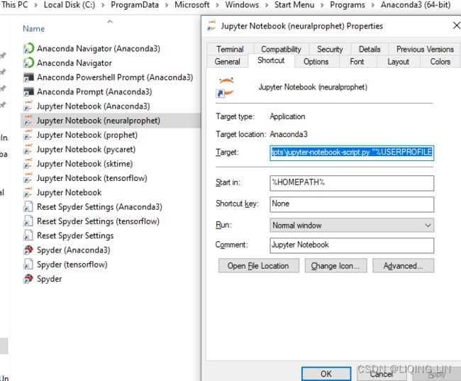 set the value of Target:
C:\ProgramData\Anaconda3\python.exe C:\ProgramData\Anaconda3\cwp.py C:\ProgramData\Anaconda3\envs\neuralprophet C:\ProgramData\Anaconda3\envs\neuralprophet\python.exe C:\ProgramData\Anaconda3\envs\neuralprophet\Scripts\jupyter-notebook-script.py "%USERPROFILE%/"vs sktime or prophet:
C:\ProgramData\Anaconda3\python.exe C:\ProgramData\Anaconda3\cwp.py C:\ProgramData\Anaconda3\envs\sktime C:\ProgramData\Anaconda3\envs\sktime\python.exe C:\ProgramData\Anaconda3\envs\sktime\Scripts\jupyter-notebook-script.py "%USERPROFILE%/"

C:\ProgramData\Anaconda3\python.exe C:\ProgramData\Anaconda3\cwp.py C:\ProgramData\Anaconda3\envs\prophet C:\ProgramData\Anaconda3\envs\prophet\python.exe C:\ProgramData\Anaconda3\envs\prophet\Scripts\jupyter-notebook-script.py "%USERPROFILE%/"
If you need additional libraries to install – for example, statsmodels – you can use pip
pip install statsmodels then create a file ![]() in the folder C:\ProgramData\Anaconda3\envs\neuralprophet\Scripts
in the folder C:\ProgramData\Anaconda3\envs\neuralprophet\Scripts
# -*- coding: utf-8 -*-
import re
import sys

from notebook.notebookapp import main

if __name__ == '__main__':
    sys.argv[0] = re.sub(r'(-script\.pyw?|\.exe)?$', '', sys.argv[0])
sys.exit(main()) 


If you need additional libraries to install – for example, statsmodels – you can use pip
pip install statsmodels
pip install lttbc
NeuralProphet makes it easy to transition from Prophet, as they follow a very similar framework for training the model
1. Start by importing the library:
from neuralprophet import NeuralProphet

import pandas as pd

# from pathlib import Path

# folder = Path('./archive/')
# aep_file = folder.joinpath('AEP_hourly.csv')
# aep = pd.read_csv( aep_file,# American Electric Power
#                    index_col='Datetime',
#                    parse_dates=True
#                  )

base='https://raw.githubusercontent.com/PacktPublishing/Time-Series-Analysis-with-Python-Cookbook/main/datasets/Ch15/'

aep = pd.read_csv( base+'AEP_hourly.csv',# American Electric Power
                   index_col='Datetime',
                   parse_dates=True
                 )
aep_cp = aep.copy(deep=True)        #####
aep_cp.sort_index(inplace=True)     ##### sort the index
aep_cp = aep_cp.resample('H').max() ##### resample
#Forward filling: ffill or pad ,
#uses the last value before the missing spot(s) and fills the gaps forward
aep_cp.ffill(inplace=True)
aep_cp.columns = ['y']              ##### rename
aep_cp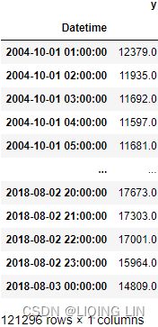
2. You will use the same energy dataset created in the Forecasting time series with multiple seasonal patterns using Prophet recipe. Instead of splitting the dataset into train and test sets, you will split into train, validation, and test sets. The validation set will be used during the training process to evaluate at every epoch:
day = 24                 # 24 hours
week = day*7             # 168 hours
month = round(week*4.35) # 731 hours
year = round(month*12)   # 8772 hours

energy = aep_cp.copy(deep=True)
energy.reset_index(inplace=True)
energy.columns = ['ds', 'y']

train = energy.iloc[:-month*2]
val = energy.iloc[-month*2:-month]
test = energy.iloc[-month:]
train
3. You will create an instance of the NeuralProphet class with default parameters.
Similar to Prophet, NeuralProphet also decomposes a time series into its components. NeuralProphet can include diferent terms such as trend, seasonality,
autoregression (the n_lags parameterModelling Auto-Regression - NeuralProphet documentation
m = NeuralProphet(
    n_forecasts=3,
    n_lags=5,
    yearly_seasonality=False,
    weekly_seasonality=False,
    daily_seasonality=False,
)
In the above example, we create a forecasting scenario which feeds 5 lags into AR-Net and receives 3 steps as forecasts. Once you have the AR-Net enabled, during forecasting your future_periods value should be equal to the n_forecasts value specified when creating the NeuralProphet object. Whichever value you specify for future_periods, it will be converted to the value of n_forecasts with a notice to the user. This is because, since the AR-Net is built during training such that it has an ouptut size of n_forecasts, it cannot support any other value during testing.),
special events (the add_events method:Modelling Events - NeuralProphet documentation
You can also provide windows for events. This way, you can consider the days around a particular event also as special events by providing the arguments lower_window and upper_window as appropriate to the add_events function of the NeuralProphet object. By default, the values for these windows are 0, which means windows are not considered.
m = NeuralProphet(
        n_forecasts=10,
        yearly_seasonality=False,
        weekly_seasonality=False,
        daily_seasonality=False,
    )
m = m.add_events(["superbowl", "playoff"], lower_window=-1, upper_window=1)

#convert the events data in the previously created dataframes into the binary input data expected by the model.
history_df = m.create_df_with_events(df, history_events_df)
According to this specification, for both superbowl and playoff events, three special events will be modelled, the event date, the previous day and the next day.
In the parameters plot too, there will now be superbowl_+1 and superbowl_-1 which correspond to the coefficients of the day following and previous to the superbowl event. The playoff event also has the same new coefficients.
# https://neuralprophet.com/tutorials/events.html#country-specific-holidays
m = m.add_events("superbowl", lower_window=-1, upper_window=1)
m = m.add_events("playoff", upper_window=2)),
future regressors (exogenous variables with the add_future_regressor methodModelling Future Regressors - NeuralProphet documentation
The default mode for future regressors in neural_prophet is additive. The regressors have to be added to the NeuralProphet object by calling the add_future_regressor function. Once this is done, the model can be fitted by providing to the fit function, the dataframe of the training data as well as the regressor values
m = NeuralProphet(
        n_forecasts=10,
        yearly_seasonality=False,
        weekly_seasonality=False,
        daily_seasonality=False,
    )

m = m.add_future_regressor(name='A', mode="multiplicative")
m = m.add_future_regressor(name='B', regularization=0.02) # Additive Future Regressors
#This will add sparsity into the individual regressor coefficients.

# df['A'] = df['y'].rolling(7, min_periods=1).mean()
# df['B'] = df['y'].rolling(30, min_periods=1).mean()
metrics = m.fit(df)
forecast = m.predict(df)
),
and lagged regressors (the add_lagged_regressor method In this example, we have a Lagged Regressor named
 A. You also need to register these Lagged Regressors with the NeuralProphet object by calling the add_lagged_regressor function and giving the necessary configs.
m = m.add_lagged_regressor(names='A')Modelling Lagged Regressors - NeuralProphet documentation). The autoregression piece is based on AR-Net, an autoregressive neural network. NeuralProphet allows you to add recurring special events – for example, a Superbowl game or a birthday. The time series modeling process is similar to that in Prophet, which was made by design. Keep in mind that NeuralProphet was built from the ground up, leveraging PyTorch, and is not a wrapper to Prophet.
# https://github.com/ourownstory/neural_prophet/blob/main/neuralprophet/forecaster.py
class NeuralProphet:
"""NeuralProphet forecaster.
A simple yet powerful forecaster that models:
Trend, seasonality, events, holidays, auto-regression, lagged covariates, and future-known regressors.
Can be regularized and configured to model nonlinear relationships.
Parameters
----------
COMMENT
Trend Config
COMMENT
growth : {'off' or 'linear'}, default 'linear'
Set use of trend growth type.
Options:
* ``off``: no trend.
* (default) ``linear``: fits a piece-wise linear trend with ``n_changepoints + 1`` segments
* ``discontinuous``: For advanced users only - not a conventional trend,
allows arbitrary jumps at each trend changepoint
changepoints : {list of str, list of np.datetimes or np.array of np.datetimes}, optional
Manually set dates at which to include potential changepoints.
Note
----
Does not accept ``np.array`` of ``np.str``. If not specified, potential changepoints are selected automatically.
n_changepoints : int
Number of potential trend changepoints to include.
Note
----
Changepoints are selected uniformly from the first ``changepoint_range`` proportion of the history.
Ignored if manual ``changepoints`` list is supplied.
changepoints_range : float
Proportion of history in which trend changepoints will be estimated.
e.g. set to 0.8 to allow changepoints only in the first 80% of training data.
Ignored if manual ``changepoints`` list is supplied.
trend_reg : float, optional
Parameter modulating the flexibility of the automatic changepoint selection.
Note
----
Large values (~1-100) will limit the variability of changepoints.
Small values (~0.001-1.0) will allow changepoints to change faster.
default: 0 will fully fit a trend to each segment.
trend_reg_threshold : bool, optional
Allowance for trend to change without regularization.
Options
* ``True``: Automatically set to a value that leads to a smooth trend.
* (default) ``False``: All changes in changepoints are regularized
trend_global_local : str, default 'global'
Modelling strategy of the trend when multiple time series are present.
Options:
* ``global``: All the elements are modelled with the same trend.
* ``local``: Each element is modelled with a different trend.
Note
----
When only one time series is input, this parameter should not be provided.
Internally it will be set to ``global``, meaning that all the elements(only one in this case)
are modelled with the same trend.
COMMENT
Seasonality Config
COMMENT
yearly_seasonality : bool, int
Fit yearly seasonality.
Options
* ``True`` or ``False``
* ``auto``: set automatically
* ``value``: number of Fourier/linear terms to generate
weekly_seasonality : bool, int
Fit monthly seasonality.
Options
* ``True`` or ``False``
* ``auto``: set automatically
* ``value``: number of Fourier/linear terms to generate
daily_seasonality : bool, int
Fit daily seasonality.
Options
* ``True`` or ``False``
* ``auto``: set automatically
* ``value``: number of Fourier/linear terms to generate
seasonality_mode : str
Specifies mode of seasonality
Options
* (default) ``additive``
* ``multiplicative``
seasonality_reg : float, optional
Parameter modulating the strength of the seasonality model.
Note
----
Smaller values (~0.1-1) allow the model to fit larger seasonal fluctuations,
larger values (~1-100) dampen the seasonality.
default: None, no regularization
season_global_local : str, default 'global'
Modelling strategy of the seasonality when multiple time series are present.
Options:
* ``global``: All the elements are modelled with the same seasonality.
* ``local``: Each element is modelled with a different seasonality.
Note
----
When only one time series is input, this parameter should not be provided.
Internally it will be set to ``global``, meaning that all the elements(only one in this case)
are modelled with the same seasonality.
COMMENT
AR Config
COMMENT
n_lags : int
Previous time series steps to include in auto-regression. Aka AR-order
ar_reg : float, optional
how much sparsity to induce in the AR-coefficients
Note
----
Large values (~1-100) will limit the number of nonzero coefficients dramatically.
Small values (~0.001-1.0) will allow more non-zero coefficients.
default: 0 no regularization of coefficients.
COMMENT
Model Config
COMMENT
n_forecasts : int
Number of steps ahead of prediction time step to forecast.
num_hidden_layers : int, optional
number of hidden layer to include in AR-Net (defaults to 0)
d_hidden : int, optional
dimension of hidden layers of the AR-Net. Ignored if ``num_hidden_layers`` == 0.
COMMENT
Train Config
COMMENT
learning_rate : float
Maximum learning rate setting for 1cycle policy scheduler.
Note
----
Default ``None``: Automatically sets the ``learning_rate`` based on a learning rate range test.
For manual user input, (try values ~0.001-10).
epochs : int
Number of epochs (complete iterations over dataset) to train model.
Note
----
Default ``None``: Automatically sets the number of epochs based on dataset size.
For best results also leave batch_size to None. For manual values, try ~5-500.
batch_size : int
Number of samples per mini-batch.
If not provided, ``batch_size`` is approximated based on dataset size.
For manual values, try ~8-1024.
For best results also leave ``epochs`` to ``None``.
newer_samples_weight: float, default 2.0
Sets factor by which the model fit is skewed towards more recent observations.
Controls the factor by which final samples are weighted more compared to initial samples.
Applies a positional weighting to each sample's loss value.
e.g. ``newer_samples_weight = 2``: final samples are weighted twice as much as initial samples.
newer_samples_start: float, default 0.0
Sets beginning of 'newer' samples as fraction of training data.
Throughout the range of 'newer' samples, the weight is increased
from ``1.0/newer_samples_weight`` initially to 1.0 at the end,
in a monotonously increasing function (cosine from pi to 2*pi).
loss_func : str, torch.nn.functional.loss
Type of loss to use:
Options
* (default) ``Huber``: Huber loss function
* ``MSE``: Mean Squared Error loss function
* ``MAE``: Mean Absolute Error loss function
* ``torch.nn.functional.loss.``: loss or callable for custom loss, eg. L1-Loss
Examples
--------
>>> from neuralprophet import NeuralProphet
>>> import torch
>>> import torch.nn as nn
>>> m = NeuralProphet(loss_func=torch.nn.L1Loss)
collect_metrics : list of str, dict, bool
Set metrics to compute.
Options
* (default) ``True``: [``mae``, ``rmse``]
* ``False``: No metrics
* ``list``: Valid options: [``mae``, ``rmse``, ``mse``]
* ``dict``: Collection of torchmetrics.Metric objects
Examples
--------
>>> from neuralprophet import NeuralProphet
>>> m = NeuralProphet(collect_metrics=["MSE", "MAE", "RMSE"])
COMMENT
Uncertainty Estimation
COMMENT
quantiles : list, default None
A list of float values between (0, 1) which indicate the set of quantiles to be estimated.
COMMENT
Missing Data
COMMENT
impute_missing : bool
whether to automatically impute missing dates/values
Note
----
imputation follows a linear method up to 20 missing values, more are filled with trend.
impute_linear : int
maximal number of missing dates/values to be imputed linearly (default: ``10``)
impute_rolling : int
maximal number of missing dates/values to be imputed
using rolling average (default: ``10``)
drop_missing : bool
whether to automatically drop missing samples from the data
Options
* (default) ``False``: Samples containing NaN values are not dropped.
* ``True``: Any sample containing at least one NaN value will be dropped.
COMMENT
Data Normalization
COMMENT
normalize : str
Type of normalization to apply to the time series.
Options
* ``off`` bypasses data normalization
* (default, binary timeseries) ``minmax`` scales the minimum value to 0.0 and the maximum value to 1.0
* ``standardize`` zero-centers and divides by the standard deviation
* (default) ``soft`` scales the minimum value to 0.0 and the 95th quantile to 1.0
* ``soft1`` scales the minimum value to 0.1 and the 90th quantile to 0.9
global_normalization : bool
Activation of global normalization
Options
* ``True``: dict of dataframes is used as global_time_normalization
* (default) ``False``: local normalization
global_time_normalization : bool
Specifies global time normalization
Options
* (default) ``True``: only valid in case of global modeling local normalization
* ``False``: set time data_params locally
unknown_data_normalization : bool
Specifies unknown data normalization
Options
* ``True``: test data is normalized with global data params even if trained with local data params (global modeling with local normalization)
* (default) ``False``: no global modeling with local normalization
accelerator: str
Name of accelerator from pytorch_lightning.accelerators to use for training. Use "auto" to automatically select an available accelerator.
Provide `None` to deactivate the use of accelerators.
trainer_config: dict
Dictionary of additional trainer configuration parameters.
"""
model: time_net.TimeNet
trainer: pl.Trainer
def __init__(
self,
growth: np_types.GrowthMode = "linear",
changepoints: Optional[list] = None,
n_changepoints: int = 10,
changepoints_range: float = 0.8,
trend_reg: float = 0,
trend_reg_threshold: Optional[Union[bool, float]] = False,
trend_global_local: str = "global",
yearly_seasonality: np_types.SeasonalityArgument = "auto",
weekly_seasonality: np_types.SeasonalityArgument = "auto",
daily_seasonality: np_types.SeasonalityArgument = "auto",
seasonality_mode: np_types.SeasonalityMode = "additive",
seasonality_reg: float = 0,
season_global_local: np_types.SeasonGlobalLocalMode = "global",
n_forecasts: int = 1,
n_lags: int = 0,
num_hidden_layers: int = 0,
d_hidden: Optional[int] = None,
ar_reg: Optional[float] = None,
learning_rate: Optional[float] = None,
epochs: Optional[int] = None,
batch_size: Optional[int] = None,
loss_func: Union[str, torch.nn.modules.loss._Loss, Callable] = "Huber",
optimizer: Union[str, Type[torch.optim.Optimizer]] = "AdamW",
newer_samples_weight: float = 2,
newer_samples_start: float = 0.0,
quantiles: List[float] = [],
impute_missing: bool = True,
impute_linear: int = 10,
impute_rolling: int = 10,
drop_missing: bool = False,
collect_metrics: np_types.CollectMetricsMode = True,
normalize: np_types.NormalizeMode = "auto",
global_normalization: bool = False,
global_time_normalization: bool = True,
unknown_data_normalization: bool = False,
accelerator: Optional[str] = None,
trainer_config: dict = {},
):
# General
self.name = "NeuralProphet"
self.n_forecasts = n_forecasts
# Data Normalization settings
self.config_normalization = configure.Normalization(
normalize=normalize,
global_normalization=global_normalization,
global_time_normalization=global_time_normalization,
unknown_data_normalization=unknown_data_normalization,
)
# Missing Data Preprocessing
self.config_missing = configure.MissingDataHandling(
impute_missing=impute_missing,
impute_linear=impute_linear,
impute_rolling=impute_rolling,
drop_missing=drop_missing,
)
# Training
self.config_train = configure.Train(
quantiles=quantiles,
learning_rate=learning_rate,
epochs=epochs,
batch_size=batch_size,
loss_func=loss_func,
optimizer=optimizer,
newer_samples_weight=newer_samples_weight,
newer_samples_start=newer_samples_start,
trend_reg_threshold=trend_reg_threshold,
)
if isinstance(collect_metrics, list):
log.info(
DeprecationWarning(
"Providing metrics to collect via `collect_metrics` in NeuralProphet is deprecated and will be removed in a future version. The metrics are now configure in the `fit()` method via `metrics`."
)
)
self.metrics = utils_metrics.get_metrics(collect_metrics)
# AR
self.config_ar = configure.AR(
n_lags=n_lags,
ar_reg=ar_reg,
)
self.n_lags = self.config_ar.n_lags
self.max_lags = self.n_lags
# Model
self.config_model = configure.Model(
num_hidden_layers=num_hidden_layers,
d_hidden=d_hidden,
)
# Trend
self.config_trend = configure.Trend(
growth=growth,
changepoints=changepoints,
n_changepoints=n_changepoints,
changepoints_range=changepoints_range,
trend_reg=trend_reg,
trend_reg_threshold=trend_reg_threshold,
trend_global_local=trend_global_local,
)
# Seasonality
self.config_seasonality = configure.ConfigSeasonality(
mode=seasonality_mode,
reg_lambda=seasonality_reg,
yearly_arg=yearly_seasonality,
weekly_arg=weekly_seasonality,
daily_arg=daily_seasonality,
global_local=season_global_local,
condition_name=None,
)
# Events
self.config_events: Optional[configure.ConfigEvents] = None
self.config_country_holidays: Optional[configure.ConfigCountryHolidays] = None
# Extra Regressors
self.config_lagged_regressors: Optional[configure.ConfigLaggedRegressors] = None
self.config_regressors: Optional[configure.ConfigFutureRegressors] = None
# set during fit()
self.data_freq = None
# Set during _train()
self.fitted = False
self.data_params = None
# Pytorch Lightning Trainer
self.metrics_logger = MetricsLogger(save_dir=os.getcwd())
self.accelerator = accelerator
self.trainer_config = trainer_config
# set during prediction
self.future_periods = None
self.predict_steps = self.n_forecasts
# later set by user (optional)
self.highlight_forecast_step_n = None
self.true_ar_weights = None
def fit(
self,
df: pd.DataFrame,
freq: str = "auto",
validation_df: Optional[pd.DataFrame] = None,
epochs: Optional[int] = None,
batch_size: Optional[int] = None,
learning_rate: Optional[float] = None,
early_stopping: bool = False,
minimal: bool = False,
metrics: Optional[np_types.CollectMetricsMode] = None,
progress: Optional[str] = "bar",
checkpointing: bool = False,
continue_training: bool = False,
num_workers: int = 0,
):
"""Train, and potentially evaluate model.
Training/validation metrics may be distorted in case of auto-regression,
if a large number of NaN values are present in df and/or validation_df.
Parameters
----------
df : pd.DataFrame
containing column ``ds``, ``y``, and optionally``ID`` with all data
freq : str
Data step sizes. Frequency of data recording,
Note
----
Any valid frequency for pd.date_range, such as ``5min``, ``D``, ``MS`` or ``auto`` (default) to automatically set frequency.
validation_df : pd.DataFrame, dict
If provided, model with performance will be evaluated after each training epoch over this data.
epochs : int
Number of epochs to train for. If None, uses the number of epochs specified in the model config.
batch_size : int
Batch size for training. If None, uses the batch size specified in the model config.
learning_rate : float
Learning rate for training. If None, uses the learning rate specified in the model config.
early_stopping : bool
Flag whether to use early stopping to stop training when training / validation loss is no longer improving.
minimal : bool
Minimal mode deactivates metrics, the progress bar and checkpointing. Control more granular by using the `metrics`, `progress` and `checkpointing` parameters.
metrics : bool
Flag whether to collect metrics during training. If None, uses the metrics specified in the model config.
progress : str
Flag whether to show a progress bar during training. If None, uses the progress specified in the model config.
Options
* (default) ``bar``
* ``plot``
* `None`
checkpointing : bool
Flag whether to save checkpoints during training
continue_training : bool
Flag whether to continue training from the last checkpoint
num_workers : int
Number of workers for data loading. If 0, data will be loaded in the main process.
Note: using multiple workers and therefore distributed training might significantly increase
the training time since each batch needs to be copied to each worker for each epoch. Keeping
all data on the main process might be faster for most datasets.
Returns
-------
pd.DataFrame
metrics with training and potentially evaluation metrics
"""
# Configuration
if epochs is not None:
self.config_train.epochs = epochs
if batch_size is not None:
self.config_train.batch_size = batch_size
if learning_rate is not None:
self.config_train.learning_rate = learning_rate
if early_stopping is not None:
self.early_stopping = early_stopping
if metrics is not None:
self.metrics = utils_metrics.get_metrics(metrics)
# Warnings
if early_stopping:
reg_enabled = utils.check_for_regularization(
[
self.config_seasonality,
self.config_regressors,
self.config_ar,
self.config_events,
self.config_country_holidays,
self.config_trend,
self.config_lagged_regressors,
]
)
if reg_enabled:
log.warning(
"Early stopping is enabled, but regularization only starts after half the number of configured epochs. \
If you see no impact of the regularization, turn off the early_stopping or reduce the number of epochs to train for."
)
if progress == "plot" and metrics is False:
log.warning("Progress plot requires metrics to be enabled. Enabling the default metrics.")
metrics = utils_metrics.get_metrics(True)
if not self.config_normalization.global_normalization:
log.warning("When Global modeling with local normalization, metrics are displayed in normalized scale.")
if minimal:
checkpointing = False
self.metrics = False
progress = None
# Setup
# List of different time series IDs, for global-local modelling (if enabled)
df, _, _, self.id_list = df_utils.prep_or_copy_df(df)
# When only one time series is input, self.id_list = ['__df__']
self.num_trends_modelled = len(self.id_list) if self.config_trend.trend_global_local == "local" else 1
self.num_seasonalities_modelled = len(self.id_list) if self.config_seasonality.global_local == "local" else 1
self.meta_used_in_model = self.num_trends_modelled != 1 or self.num_seasonalities_modelled != 1
if self.fitted is True and not continue_training:
log.error("Model has already been fitted. Re-fitting may break or produce different results.")
self.max_lags = df_utils.get_max_num_lags(self.config_lagged_regressors, self.n_lags)
if self.max_lags == 0 and self.n_forecasts > 1:
self.n_forecasts = 1
self.predict_steps = 1
log.warning(
"Changing n_forecasts to 1. Without lags, the forecast can be "
"computed for any future time, independent of lagged values"
)
# Pre-processing
df, _, _, _ = df_utils.prep_or_copy_df(df)
df = self._check_dataframe(df, check_y=True, exogenous=True)
self.data_freq = df_utils.infer_frequency(df, n_lags=self.max_lags, freq=freq)
df = self._handle_missing_data(df, freq=self.data_freq)
# Training
if validation_df is None:
metrics_df = self._train(
df,
progress_bar_enabled=bool(progress),
metrics_enabled=bool(self.metrics),
checkpointing_enabled=checkpointing,
continue_training=continue_training,
num_workers=num_workers,
)
else:
df_val, _, _, _ = df_utils.prep_or_copy_df(validation_df)
df_val = self._check_dataframe(df_val, check_y=False, exogenous=False)
df_val = self._handle_missing_data(df_val, freq=self.data_freq)
metrics_df = self._train(
df,
df_val=df_val,
progress_bar_enabled=bool(progress),
metrics_enabled=bool(self.metrics),
checkpointing_enabled=checkpointing,
continue_training=continue_training,
num_workers=num_workers,
)
# Show training plot
if progress == "plot":
assert metrics_df is not None
if validation_df is None:
fig = pyplot.plot(metrics_df[["Loss"]])
else:
fig = pyplot.plot(metrics_df[["Loss", "Loss_val"]])
# Only display the plot if the session is interactive, eg. do not show in github actions since it
# causes an error in the Windows and MacOS environment
if matplotlib.is_interactive():
fig
self.fitted = True
return metrics_df
You will use the fit method, passing both the train and val sets:
model_np = NeuralProphet()
metrics = model_np.fit( train, validation_df=val )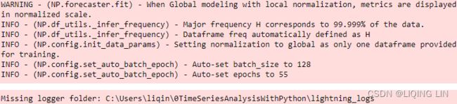 4. Similar to Prophet, you will use the make_future_dataframe method to extend the train DataFrame forward for a specific number of periods and at a specified frequency. In this case, it will be the total number of test and val observations:
n = len(test) + len(val)

future = model_np.make_future_dataframe(df=train, periods=n)
forecast = model_np.predict(df=future)
forecast 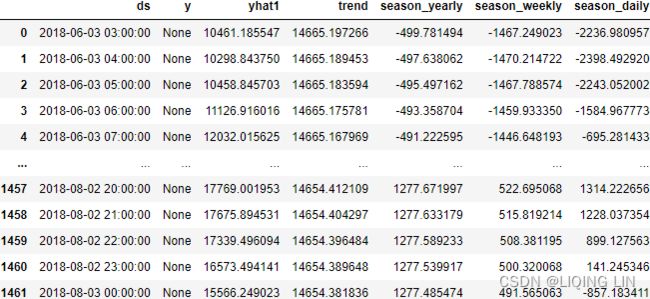

######
n = len(test) + len(val)
future = model_np.make_future_dataframe(df=train, periods=n, n_historic_predictions=True)
forecast = model_np.predict(df=future)
forecast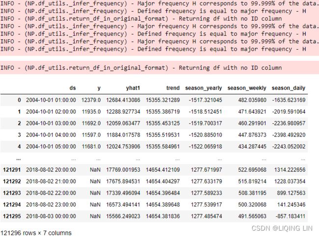
######
fig = model_np.plot(forecast,plotting_backend = 'matplotlib') # plotting_backend = 'matplotlib'(default) or 'plotly'
fig.show()
######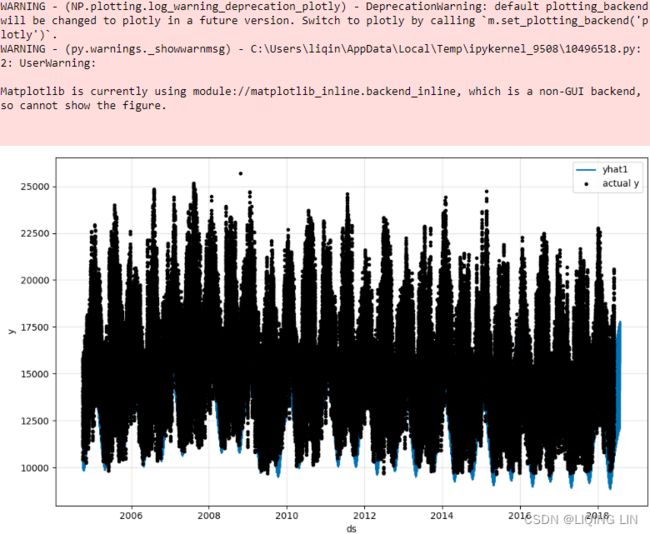
######
model_np.set_plotting_backend('plotly')
# https://github.com/ourownstory/neural_prophet/blob/main/neuralprophet/forecaster.py
#         Parameters
#         ----------
#             fcst : pd.DataFrame
#                 output of self.predict.
#             df_name : str
#                 ID from time series that should be plotted
#             ax : matplotlib axes
#                 optional, matplotlib axes on which to plot.
#             xlabel : string
#                 label name on X-axis
#             ylabel : string
#                 label name on Y-axis
#             figsize : tuple
#                 width, height in inches. default: (10, 6)
#             plotting_backend : str
#                 optional, overwrites the default plotting backend.
#                 Options
#                 * ``plotly``: Use plotly for plotting
#                 * ``matplotlib``: use matplotlib for plotting
#                 * (default) ``default``: use the global default for plotting
#             forecast_in_focus: int
#                 optinal, i-th step ahead forecast to plot
#                 Note
#                 ----
#                 None (default): plot self.highlight_forecast_step_n by default
#         """
fig = model_np.plot(forecast, figsize=(14, 8))
fig.show()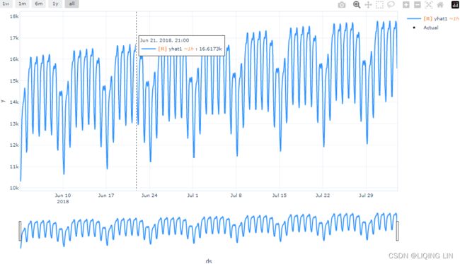
######
######
5. You plot the components using the plot_components method:
fig = model_np.plot_components(forecast, figsize=(10,8),plotting_backend='matplotlib')
fig.show()
This should produce four subplots for trend and one for each seasonal pattern (daily, weekly, and yearly). The following only shows the seasonal components:
 Figure 15.14 – The time series seasonal components automatically detected by NeuralProphet
######
import matplotlib.dates as mdates
import matplotlib.pyplot as plt

fig, axes = plt.subplots( 4,1, figsize=(12, 12) )

axes[0].plot( forecast['ds'], forecast['trend'] )
axes[0].set_xlabel('ds')
axes[0].set_ylabel('Trend')

week_select=forecast[('2018-06-03' <=forecast['ds']) & (forecast['ds']<='2018-06-10')]
axes[1].plot( week_select['ds'], week_select['season_weekly'] )
axes[1].xaxis.set_major_formatter( mdates.DateFormatter('%A') )
axes[1].set_xlabel('Day of week')
axes[1].set_ylabel('Seasonality: weekly')

year_select=forecast[('2018'<=forecast['ds']) & (forecast['ds']<'2019') ]
#year_select.set_index('ds', inplace=True)
#year_select['month'] = year_select.index.strftime(date_format='%B %-d')
axes[2].plot( year_select['ds'], year_select['season_yearly'] )
axes[2].xaxis.set_major_formatter( mdates.DateFormatter('%B %d') )
axes[2].set_xlabel('Day of year')
axes[2].set_ylabel('Seasonality: yearly')

axes[3].plot( forecast[:day]['ds'], forecast[:day]['season_daily'])
axes[3].xaxis.set_major_formatter( mdates.DateFormatter('%H:%M:%S') )
axes[3].set_xlabel('Hour of day')
axes[3].set_ylabel('Seasonality: daily')

plt.subplots_adjust(hspace = 0.4)
plt.show()
######
6. NeuralProphet provides the plot_parameters method, which gives more insight into the individual coefficients for the significant changepoints – for example, trend changepoints:
#     def plot_parameters(
#         self,
#         weekly_start=0,#0 (default) starts the week on Sunday. 1 shifts by 1 day to Monday, and so on
#         yearly_start=0,#0 (default) starts the year on Jan 1. 1 shifts by 1 day to Jan 2, and so on.
#         figsize=None,
#         forecast_in_focus=None,
#         df_name=None,
#         plotting_backend="default",
#         quantile=None,#None (default):  Parameters will be plotted for the median quantile.
#         components=None,#str or list
#                 * (default) ``None``:  All parameter the user set in the model configuration are plotted.
#                 * ``trend``
#                 * ``trend_rate_change``
#                 * ``seasonality``: : select all seasonalities
#                 * ``autoregression``
#                 * ``lagged_regressors``: select all lagged regressors
#                 * ``events``: select all events and country holidays
#                 * ``future_regressors``: select all future regressors
#     ):

fig = model_np.plot_parameters()
fig.show()
Figure 15.15 – Trend changepoints affecting the overall trend

7. Compare the out-of-sample prediction values with the test dataset:
forecast.set_index('ds')['yhat1'].iloc[-month:] 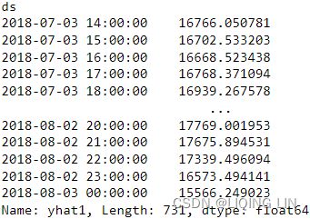 vs
vs
forecast.set_index('ds')['yhat1'].iloc[-month*2:-month]  vs
vs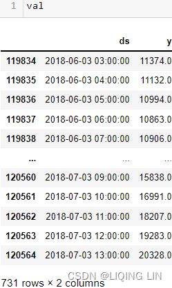
prediction = forecast.set_index('ds').loc['2018-07-03 14:00:00':]['yhat1']

test.set_index('ds').plot( style='k--', alpha=0.5, figsize=(12,6) )
prediction.plot(style='k')
plt.legend(['Actual', 'Predicted'])
plt.title('Out-of-Sample Forecast: Actual vs Predicted')
plt.show()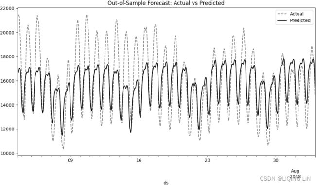
Figure 15.16 – Actual versus Predicted with NeuralProphet
Compare Figure 15.16 with Figure 15.11. They look similar, which is why you will need to capture some metrics to quantify the performance and make it easier to compare the two models.
8. Calculate both RMSE and RMSPE:
from statsmodels.tools.eval_measures import rmse, rmspe

rmspe(test['y'].values, prediction.values) 
rmse(test['y'].values, prediction.values) ![]()
Overall, both RMSE and RMSPE for NeuralProphet indicate that the model outperforms Prophet(RMSE: and RMSPE:![]() ).
).
NeuralProphet offers fexibility and extensibility (and is very modular for anyone that wants to extend its capabilities). The library also provides additional features tailored专门制作,定制的 to working with deep neural networks, such as logging performance, cross-validation, spitting data, benchmarking, and experimentation.
Let's explore some of these features.
You can change the learning rate when you first initialize the model, and use the split_df method to split data into train and test sets. You can also specify a holdout portion (a percentage from the train set) to be used for validation on each epoch:
from neuralprophet import NeuralProphet, set_log_level

set_log_level('ERROR')
The validation is set at 20% (0. 2) of the training set.
m = NeuralProphet(learning_rate=0.1)

train, test = m.split_df( df=energy, freq='H', valid_p=0.2 )

train_results = m.fit(df=train, freq='H')

test_results = m.test(df=test) # """Evaluate model on holdout data.
test_results
Using the test method, you can get the scores against the test set:
train_results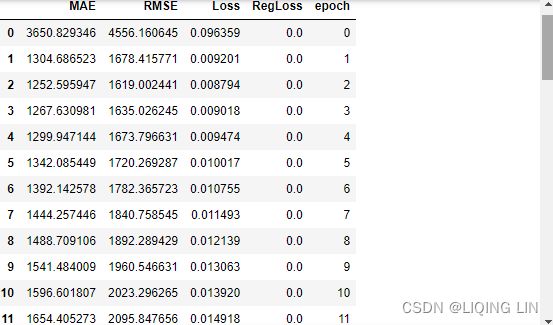
...
train_results contains the scores for each epoch. You can instruct NeuralProphet to plot these:
m = NeuralProphet(learning_rate=0.1)

train, test = m.split_df( df=energy, freq='H', valid_p=0.2 )

metrics = m.fit(df=train, freq='H', validation_df=test,
                progress="plot"
               )
This will refresh the plot on each iteration so that you can see how the model is learning during the fitting (training) process. This way, you do not have to wait until the training is complete. The following is a snapshot during training:
 Figure 15.17 – NeuralProphet allows you to visualize performance while training
Once training is complete (in this case, at the 57 epoch), the plot will show the final output at all epochs. You can print the last 5 rows, as shown in the following code block:
metrics.tail(n=5) To learn more about NeuralProphet, you can reference the offcial documentation here: NeuralProphet documentation