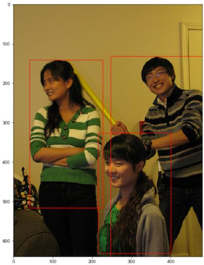
x y x y xyxy xyxy,即 ( x 1 , y 1 , x 2 , y 2 ) (x_1, y_1, x_2, y_2) (x1,y1,x2,y2),其中 ( x 1 , y 1 ) (x_1, y_1) (x1,y1)是矩形框左上角的坐标, ( x 2 , y 2 ) (x_2, y_2) (x2,y2)是矩形框右下角的坐标。图4中3个红色矩形框用xyxy格式表示如下:
x y w h xywh xywh,即 ( x , y , w , h ) (x, y, w, h) (x,y,w,h),其中 ( x , y ) (x, y) (x,y)是矩形框中心点的坐标, w w w是矩形框的宽度, h h h是矩形框的高度。
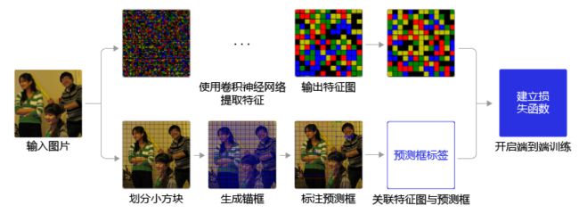
在检测任务中,训练数据集的标签里会给出目标物体真实边界框所对应的 ( x 1 , y 1 , x 2 , y 2 ) (x_1, y_1, x_2, y_2) (x1,y1,x2,y2),这样的边界框也被称为真实框(ground truth box),如 图4 所示,图中画出了3个人像所对应的真实框。模型会对目标物体可能出现的位置进行预测,由模型预测出的边界框则称为预测框(prediction box)。
注意:
在阅读代码时,请注意使用的是哪一种格式的表示方式。
图片坐标的原点在左上角, x x x轴向右为正方向, y y y轴向下为正方向。
要完成一项检测任务,我们通常希望模型能够根据输入的图片,输出一些预测的边界框,以及边界框中所包含的物体的类别或者说属于某个类别的概率,例如这种格式: [ L , P , x 1 , y 1 , x 2 , y 2 ] [L, P, x_1, y_1, x_2, y_2] [L,P,x1,y1,x2,y2],其中 L L L是类别标签, P P P是物体属于该类别的概率。一张输入图片可能会产生多个预测框,接下来让我们一起学习如何完成这项任务。
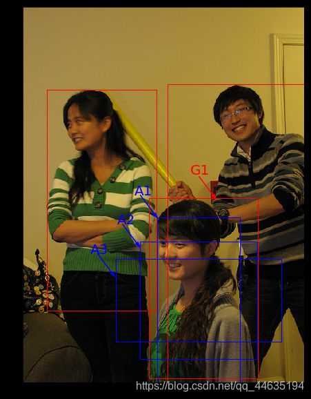
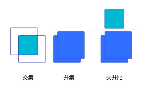
上面我们画出了以点 ( 300 , 500 ) (300, 500) (300,500)为中心,生成的三个锚框,我们可以看到锚框A1 与真实框 G1的重合度比较好。那么如何衡量这三个锚框跟真实框之间的关系呢?在检测任务中,使用交并比(Intersection of Union,IoU)作为衡量指标。这一概念来源于数学中的集合,用来描述两个集合 A A A和 B B B之间的关系,它等于两个集合的交集里面所包含的元素个数,除以它们的并集里面所包含的元素个数,具体计算公式如下:
I o U = A ∩ B A ∪ B IoU = \frac{A\cap B}{A \cup B} IoU=A∪BA∩B
假设两个矩形框A和B的位置分别为: A : [ x a 1 , y a 1 , x a 2 , y a 2 ] A: [x_{a1}, y_{a1}, x_{a2}, y_{a2}] A:[xa1,ya1,xa2,ya2]
B : [ x b 1 , y b 1 , x b 2 , y b 2 ] B: [x_{b1}, y_{b1}, x_{b2}, y_{b2}] B:[xb1,yb1,xb2,yb2]
假如位置关系如 图6 所示:
图6:计算交并比
如果二者有相交部分,则相交部分左上角坐标为: x 1 = m a x ( x a 1 , x b 1 ) , y 1 = m a x ( y a 1 , y b 1 ) x_1 = max(x_{a1}, x_{b1}), \ \ \ \ \ y_1 = max(y_{a1}, y_{b1}) x1=max(xa1,xb1),y1=max(ya1,yb1)
相交部分右下角坐标为: x 2 = m i n ( x a 2 , x b 2 ) , y 2 = m i n ( y a 2 , y b 2 ) x_2 = min(x_{a2}, x_{b2}), \ \ \ \ \ y_2 = min(y_{a2}, y_{b2}) x2=min(xa2,xb2),y2=min(ya2,yb2)
计算先交部分面积: i n t e r s e c t i o n = m a x ( x 2 − x 1 + 1.0 , 0 ) ⋅ m a x ( y 2 − y 1 + 1.0 , 0 ) intersection = max(x_2 - x_1 + 1.0, 0) \cdot max(y_2 - y_1 + 1.0, 0) intersection=max(x2−x1+1.0,0)⋅max(y2−y1+1.0,0)
矩形框A和B的面积分别是: S A = ( x a 2 − x a 1 + 1.0 ) ⋅ ( y a 2 − y a 1 + 1.0 ) S_A = (x_{a2} - x_{a1} + 1.0) \cdot (y_{a2} - y_{a1} + 1.0) SA=(xa2−xa1+1.0)⋅(ya2−ya1+1.0)
S B = ( x b 2 − x b 1 + 1.0 ) ⋅ ( y b 2 − y b 1 + 1.0 ) S_B = (x_{b2} - x_{b1} + 1.0) \cdot (y_{b2} - y_{b1} + 1.0) SB=(xb2−xb1+1.0)⋅(yb2−yb1+1.0)
计算相并部分面积: u n i o n = S A + S B − i n t e r s e c t i o n union = S_A + S_B - intersection union=SA+SB−intersection
计算交并比:
I o U = i n t e r s e c t i o n u n i o n IoU = \frac{intersection}{union} IoU=unionintersection
INSECT_NAMES =['Boerner','Leconte','Linnaeus','acuminatus','armandi','coleoptera','linnaeus']defget_insect_names():"""
return a dict, as following,
{'Boerner': 0,
'Leconte': 1,
'Linnaeus': 2,
'acuminatus': 3,
'armandi': 4,
'coleoptera': 5,
'linnaeus': 6
}
It can map the insect name into an integer label.
"""
insect_category2id ={}for i, item inenumerate(INSECT_NAMES):
insect_category2id[item]= i
return insect_category2id
此小方块区域左上角的位置坐标是: c x = 4 c_x = 4 cx=4 c y = 10 c_y = 10 cy=10
此锚框的区域中心坐标是: c e n t e r _ x = c x + 0.5 = 4.5 center\_x = c_x + 0.5 = 4.5 center_x=cx+0.5=4.5 c e n t e r _ y = c y + 0.5 = 10.5 center\_y = c_y + 0.5 = 10.5 center_y=cy+0.5=10.5
可以通过下面的方式生成预测框的中心坐标: b x = c x + σ ( t x ) b_x = c_x + \sigma(t_x) bx=cx+σ(tx) b y = c y + σ ( t y ) b_y = c_y + \sigma(t_y) by=cy+σ(ty)
其中 t x t_x tx和 t y t_y ty为实数, σ ( x ) \sigma(x) σ(x)是我们之前学过的Sigmoid函数,其定义如下:
σ ( x ) = 1 1 + e x p ( − x ) \sigma(x) = \frac{1}{1 + exp(-x)} σ(x)=1+exp(−x)1
这里我们会问:当 t x , t y , t w , t h t_x, t_y, t_w, t_h tx,ty,tw,th取值为多少的时候,预测框能够跟真实框重合?为了回答问题,只需要将上面预测框坐标中的 b x , b y , b h , b w b_x, b_y, b_h, b_w bx,by,bh,bw设置为真实框的位置,即可求解出 t t t的数值。
令: σ ( t x ∗ ) + c x = g t x \sigma(t^*_x) + c_x = gt_x σ(tx∗)+cx=gtx σ ( t y ∗ ) + c y = g t y \sigma(t^*_y) + c_y = gt_y σ(ty∗)+cy=gty p w e t w ∗ = g t h p_w e^{t^*_w} = gt_h pwetw∗=gth p h e t h ∗ = g t w p_h e^{t^*_h} = gt_w pheth∗=gtw
可以求解出 ( t x ∗ , t y ∗ , t w ∗ , t h ∗ ) (t^*_x, t^*_y, t^*_w, t^*_h) (tx∗,ty∗,tw∗,th∗)
如果 t t t是网络预测的输出值,将 t ∗ t^* t∗作为目标值,以他们之间的差距作为损失函数,则可以建立起一个回归问题,通过学习网络参数,使得 t t t足够接近 t ∗ t^* t∗,从而能够求解出预测框的位置坐标和大小。
预测框可以看作是在锚框基础上的一个微调,每个锚框会有一个跟它对应的预测框,我们需要确定上面计算式中的 t x , t y , t w , t h t_x, t_y, t_w, t_h tx,ty,tw,th,从而计算出与锚框对应的预测框的位置和形状。
在前面我们已经问过这样一个问题:当 t x , t y , t w , t h t_x, t_y, t_w, t_h tx,ty,tw,th取值为多少的时候,预测框能够跟真实框重合?其做法是将预测框坐标中的 b x , b y , b h , b w b_x, b_y, b_h, b_w bx,by,bh,bw设置为真实框的坐标,即可求解出 t t t的数值。
令: σ ( t x ∗ ) + c x = g t x \sigma(t^*_x) + c_x = gt_x σ(tx∗)+cx=gtx σ ( t y ∗ ) + c y = g t y \sigma(t^*_y) + c_y = gt_y σ(ty∗)+cy=gty p w e t w ∗ = g t w p_w e^{t^*_w} = gt_w pwetw∗=gtw p h e t h ∗ = g t h p_h e^{t^*_h} = gt_h pheth∗=gth
对于 t x ∗ t_x^* tx∗和 t y ∗ t_y^* ty∗,由于Sigmoid的反函数不好计算,我们直接使用 σ ( t x ∗ ) \sigma(t^*_x) σ(tx∗)和 σ ( t y ∗ ) \sigma(t^*_y) σ(ty∗)作为回归的目标。
d x ∗ = σ ( t x ∗ ) = g t x − c x d_x^* = \sigma(t^*_x) = gt_x - c_x dx∗=σ(tx∗)=gtx−cx
d y ∗ = σ ( t y ∗ ) = g t y − c y d_y^* = \sigma(t^*_y) = gt_y - c_y dy∗=σ(ty∗)=gty−cy
t w ∗ = l o g ( g t w p w ) t^*_w = log(\frac{gt_w}{p_w}) tw∗=log(pwgtw)
t h ∗ = l o g ( g t h p h ) t^*_h = log(\frac{gt_h}{p_h}) th∗=log(phgth)
如果 ( t x , t y , t h , t w ) (t_x, t_y, t_h, t_w) (tx,ty,th,tw)是网络预测的输出值,将 ( d x ∗ , d y ∗ , t w ∗ , t h ∗ ) (d_x^*, d_y^*, t_w^*, t_h^*) (dx∗,dy∗,tw∗,th∗)作为 ( σ ( t x ) , σ ( t y ) , t h , t w ) (\sigma(t_x), \sigma(t_y), t_h, t_w) (σ(tx),σ(ty),th,tw)的目标值,以它们之间的差距作为损失函数,则可以建立起一个回归问题,通过学习网络参数,使得 t t t足够接近 t ∗ t^* t∗,从而能够求解出预测框的位置。
通过这种方式,我们在每个小方块区域都生成了一系列的锚框作为候选区域,并且根据图片上真实物体的位置,标注出了每个候选区域对应的objectness标签、位置需要调整的幅度以及包含的物体所属的类别。位置需要调整的幅度由4个变量描述 ( t x , t y , t w , t h ) (t_x, t_y, t_w, t_h) (tx,ty,tw,th),objectness标签需要用一个变量描述 o b j obj obj,描述所属类别的变量长度等于类别数C。
对于每个锚框,模型需要预测输出 ( t x , t y , t w , t h , P o b j , P 1 , P 2 , . . . , P C ) (t_x, t_y, t_w, t_h, P_{obj}, P_1, P_2,... , P_C) (tx,ty,tw,th,Pobj,P1,P2,...,PC),其中 P o b j P_{obj} Pobj是锚框是否包含物体的概率, P 1 , P 2 , . . . , P C P_1, P_2,... , P_C P1,P2,...,PC则是锚框包含的物体属于每个类别的概率。接下来让我们一起学习如何通过卷积神经网络输出这样的预测值。
import paddle.fluid as fluid
from paddle.fluid.param_attr import ParamAttr
from paddle.fluid.regularizer import L2Decay
from paddle.fluid.dygraph.nn import Conv2D, BatchNorm
from paddle.fluid.dygraph.base import to_variable
# YOLO-V3骨干网络结构Darknet53的实现代码classConvBNLayer(fluid.dygraph.Layer):"""
卷积 + 批归一化,BN层之后激活函数默认用leaky_relu
"""def__init__(self,
ch_in,
ch_out,
filter_size=3,
stride=1,
groups=1,
padding=0,
act="leaky",
is_test=True):super(ConvBNLayer, self).__init__()
self.conv = Conv2D(
num_channels=ch_in,
num_filters=ch_out,
filter_size=filter_size,
stride=stride,
padding=padding,
groups=groups,
param_attr=ParamAttr(
initializer=fluid.initializer.Normal(0.,0.02)),
bias_attr=False,
act=None)
self.batch_norm = BatchNorm(
num_channels=ch_out,
is_test=is_test,
param_attr=ParamAttr(
initializer=fluid.initializer.Normal(0.,0.02),
regularizer=L2Decay(0.)),
bias_attr=ParamAttr(
initializer=fluid.initializer.Constant(0.0),
regularizer=L2Decay(0.)))
self.act = act
defforward(self, inputs):
out = self.conv(inputs)
out = self.batch_norm(out)if self.act =='leaky':
out = fluid.layers.leaky_relu(x=out, alpha=0.1)return out
classDownSample(fluid.dygraph.Layer):"""
下采样,图片尺寸减半,具体实现方式是使用stirde=2的卷积
"""def__init__(self,
ch_in,
ch_out,
filter_size=3,
stride=2,
padding=1,
is_test=True):super(DownSample, self).__init__()
self.conv_bn_layer = ConvBNLayer(
ch_in=ch_in,
ch_out=ch_out,
filter_size=filter_size,
stride=stride,
padding=padding,
is_test=is_test)
self.ch_out = ch_out
defforward(self, inputs):
out = self.conv_bn_layer(inputs)return out
classBasicBlock(fluid.dygraph.Layer):"""
基本残差块的定义,输入x经过两层卷积,然后接第二层卷积的输出和输入x相加
"""def__init__(self, ch_in, ch_out, is_test=True):super(BasicBlock, self).__init__()
self.conv1 = ConvBNLayer(
ch_in=ch_in,
ch_out=ch_out,
filter_size=1,
stride=1,
padding=0,
is_test=is_test
)
self.conv2 = ConvBNLayer(
ch_in=ch_out,
ch_out=ch_out*2,
filter_size=3,
stride=1,
padding=1,
is_test=is_test
)defforward(self, inputs):
conv1 = self.conv1(inputs)
conv2 = self.conv2(conv1)
out = fluid.layers.elementwise_add(x=inputs, y=conv2, act=None)return out
classLayerWarp(fluid.dygraph.Layer):"""
添加多层残差块,组成Darknet53网络的一个层级
"""def__init__(self, ch_in, ch_out, count, is_test=True):super(LayerWarp,self).__init__()
self.basicblock0 = BasicBlock(ch_in,
ch_out,
is_test=is_test)
self.res_out_list =[]for i inrange(1, count):
res_out = self.add_sublayer("basic_block_%d"%(i),#使用add_sublayer添加子层
BasicBlock(ch_out*2,
ch_out,
is_test=is_test))
self.res_out_list.append(res_out)defforward(self,inputs):
y = self.basicblock0(inputs)for basic_block_i in self.res_out_list:
y = basic_block_i(y)return y
DarkNet_cfg ={53:([1,2,8,8,4])}classDarkNet53_conv_body(fluid.dygraph.Layer):def__init__(self,
is_test=True):super(DarkNet53_conv_body, self).__init__()
self.stages = DarkNet_cfg[53]
self.stages = self.stages[0:5]# 第一层卷积
self.conv0 = ConvBNLayer(
ch_in=3,
ch_out=32,
filter_size=3,
stride=1,
padding=1,
is_test=is_test)# 下采样,使用stride=2的卷积来实现
self.downsample0 = DownSample(
ch_in=32,
ch_out=32*2,
is_test=is_test)# 添加各个层级的实现
self.darknet53_conv_block_list =[]
self.downsample_list =[]for i, stage inenumerate(self.stages):
conv_block = self.add_sublayer("stage_%d"%(i),
LayerWarp(32*(2**(i+1)),32*(2**i),
stage,
is_test=is_test))
self.darknet53_conv_block_list.append(conv_block)# 两个层级之间使用DownSample将尺寸减半for i inrange(len(self.stages)-1):
downsample = self.add_sublayer("stage_%d_downsample"% i,
DownSample(ch_in=32*(2**(i+1)),
ch_out=32*(2**(i+2)),
is_test=is_test))
self.downsample_list.append(downsample)defforward(self,inputs):
out = self.conv0(inputs)#print("conv1:",out.numpy())
out = self.downsample0(out)#print("dy:",out.numpy())
blocks =[]for i, conv_block_i inenumerate(self.darknet53_conv_block_list):#依次将各个层级作用在输入上面
out = conv_block_i(out)
blocks.append(out)if i <len(self.stages)-1:
out = self.downsample_list[i](out)return blocks[-1:-4:-1]# 将C0, C1, C2作为返回值
根据输出特征图计算预测框位置和类别
YOLO-V3中对每个预测框计算逻辑如下:
预测框是否包含物体。也可理解为objectness=1的概率是多少,可以用网络输出一个实数 x x x,可以用 S i g m o i d ( x ) Sigmoid(x) Sigmoid(x)表示objectness为正的概率 P o b j P_{obj} Pobj
预测物体位置和形状。物体位置和形状 t x , t y , t w , t h t_x, t_y, t_w, t_h tx,ty,tw,th可以用网络输出4个实数来表示 t x , t y , t w , t h t_x, t_y, t_w, t_h tx,ty,tw,th
预测物体类别。预测图像中物体的具体类别是什么,或者说其属于每个类别的概率分别是多少。总的类别数为C,需要预测物体属于每个类别的概率 ( P 1 , P 2 , . . . , P C ) (P_1, P_2, ..., P_C) (P1,P2,...,PC),可以用网络输出C个实数 ( x 1 , x 2 , . . . , x C ) (x_1, x_2, ..., x_C) (x1,x2,...,xC),对每个实数分别求Sigmoid函数,让 P i = S i g m o i d ( x i ) P_i = Sigmoid(x_i) Pi=Sigmoid(xi),则可以表示出物体属于每个类别的概率。
对于一个预测框,网络需要输出 ( 5 + C ) (5 + C) (5+C)个实数来表征它是否包含物体、位置和形状尺寸以及属于每个类别的概率。
由于我们在每个小方块区域都生成了K个预测框,则所有预测框一共需要网络输出的预测值数目是:
[ K ( 5 + C ) ] × m × n [K(5 + C)] \times m \times n [K(5+C)]×m×n
还有更重要的一点是网络输出必须要能区分出小方块区域的位置来,不能直接将特征图连接一个输出大小为 [ K ( 5 + C ) ] × m × n [K(5 + C)] \times m \times n [K(5+C)]×m×n的全连接层。
下面需要将像素点 ( i , j ) (i,j) (i,j)与第i行第j列的小方块区域所需要的预测值关联起来,每个小方块区域产生K个预测框,每个预测框需要 ( 5 + C ) (5 + C) (5+C)个实数预测值,则每个像素点相对应的要有 K ( 5 + C ) K(5 + C) K(5+C)个实数。为了解决这一问题,对特征图进行多次卷积,并将最终的输出通道数设置为 K ( 5 + C ) K(5 + C) K(5+C),即可将生成的特征图与每个预测框所需要的预测值巧妙的对应起来。
This article is from an interview with Zuhaib Siddique, a production engineer at HipChat, makers of group chat and IM for teams.
HipChat started in an unusual space, one you might not