基于Jaya优化算法的电力系统最优潮流研究(Matlab代码实现)
欢迎来到本博客❤️❤️
博主优势:博客内容尽量做到思维缜密,逻辑清晰,为了方便读者。
⛳️座右铭:行百里者,半于九十。
本文目录如下:
目录
1 概述
2 运行结果
3 参考文献
4 Matlab代码实现

1 概述
电力系统最优潮流是指在满足电力系统各种约束条件的前提下,使得系统的总损耗最小的潮流分布状态。最优潮流问题是电力系统运行和规划中的重要问题之一,对于确保电力系统的安全、稳定和经济运行具有重要意义。
最优潮流问题可以用一个非线性优化问题来表示,目标函数是最小化系统的总损耗,约束条件包括节点功率平衡方程、节点电压幅值和相角限制、线路功率限制等。解决最优潮流问题需要使用数学方法和计算工具,常用的方法包括牛顿-拉夫森法、潮流迭代法、内点法等。
最优潮流问题的解决可以为电力系统运行和规划提供重要的参考依据。通过调整潮流分布,可以减少系统的总损耗,提高系统的运行效率和经济性。此外,最优潮流问题还可以应用于电力市场运营、电力交易和电力系统规划等领域,为电力系统的可持续发展提供支持。
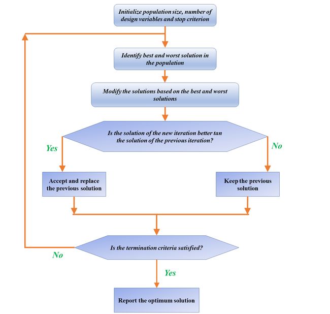
基于Jaya优化算法的电力系统最优潮流研究是一种针对电力系统进行优化设计的方法。Jaya优化算法是一种基于自然界中的蝗虫聚群行为进行优化的算法,通过模拟蝗虫在自然界中的聚群行为,寻找最优解。该算法具有收敛速度快、精度高、易于实现等优点。
在电力系统最优潮流研究中,Jaya优化算法被用于寻找电力系统中最优的电压和功率分配方案。通过对电力系统中各个节点的电压和功率进行优化,可以实现电力系统的最优化运行,提高电力系统的效率和可靠性。同时,该方法还可以实现电力系统的负荷均衡,减少电力系统的能源损耗和污染,具有重要的应用价值。
2 运行结果
主函数代码:
%+++++++++++++++++++ Data base of the power system ++++++++++++++++++++++++
% The following file contains information about the topology of the power
% system such as the bus and line matrix
data_39;
% original matrix and generation buses
bus_o=bus; line_o=line;
slack=find(bus(:,10)==1); % Slack bus
PV=find(bus(:,10)==2);   % Generation buses PV
Bgen=vertcat(slack,PV);     % Slack and PV buses
PQ=find(bus(:,10)==3);   % Load buses

% +++++++++++++++ Parameters of the optimization algorithm ++++++++++++++++
pop =  210;                                % Size of the population
n_itera = 35;                             % Number of iterations of the optimization algorithm
Vmin=0.95;                                % Minimum value of voltage for the generators
Vmax=1.05;                                % Maximum value of voltage for the generators
mini_tap = 0.95;                          % Minimum value of the TAP
maxi_tap = 1.05;                          % Maximum value of the TAP
Smin=-0.5;                                % Minimum Shunt value
Smax=0.5;                                 % Maximum Sunt value
pos_Shunt = find( bus(:,11) ~= 0);        % Positions of Shunts in bus matrix
pos_tap = find( line(:,6) ~= 0);          % Positions of TAPs in line matrix
tap_o = line(pos_tap,6);                  % Original values of TAPs
Shunt_o = bus(pos_Shunt,9);               % Original values of Shunts
n_tap = length(pos_tap);                  % number of TAPs
n_Shunt = length(pos_Shunt);              % number of Shunts
n_nodos = length(bus(:,1));               % number of buses of the power system

% ++++++++++++++++ First: Run power flow for the base case ++++++++++++++++
% Store V and theta of the base case
[V_o,Theta_o,~] = PowerFlowClassical(bus_o,line_o);
% +++++++++++++++++++Compute the active power lossess++++++++++++++++++++++
nbranch=length(line_o(:,1));
FromNode=line_o(:,1);
ToNode=line_o(:,2);
for k=1:nbranch
    a(k)=line_o(k,6);
    if a(k)==0 % in this case, we are analyzing lines
        Zpq(k)=line_o(k,3)+1i*line_o(k,4); % impedance of the transmission line
        Ypq(k)=Zpq(k)^-1; % admittance of the transmission linee
        gpq(k)=real(Ypq(k)); % conductance of the transmission line
        % Active power loss of the corresponding line
        Llpq(k)=gpq(k)*(V_o(FromNode(k))^2 +V_o(ToNode(k))^2 -2*V_o(FromNode(k))*V_o(ToNode(k))*cos(Theta_o(FromNode(k))-Theta_o(ToNode(k))));
    end
end
% Total active power lossess
Plosses=sum(Llpq);
% +++++++++++++++++++++++++++ Optimum power flow ++++++++++++++++++++++++++
% Start the population
for k=1:n_tap % Start the TAP population
    x_tap(:,k) = mini_tap +(maxi_tap - mini_tap)*(0.1*floor((10*rand(pop,1))));
end
for k=1:n_Shunt % Start the Shunt population
     x_shunt(:,k) = Smin +(Smax - Smin)*(0.1*floor((10*rand(pop,1))));
end
for k=1:length(Bgen) % Start the population of voltage from generators
    x_vg(:,k) = Vmin +(Vmax - Vmin)*(0.1*floor((10*rand(pop,1))));
end
% JAYA algorithm
for k=1:n_itera
    % with the new values of the TAPs, Shunts and VGs recompute V and Ybus
    % Modify line and bus matrix
    for p=1:pop
        for q=1:n_tap
            r=pos_tap(q);
            line(r,6)=x_tap(p,q); % modification of line matrix acording to the new TAP values
        end; clear r
        for qa=1:n_Shunt
            r=pos_Shunt(qa);
             bus(r,9)=x_shunt(p,qa); % modification of bus matrix according to the new Shunt values
        end; clear r
        for qb=1:length(Bgen)
            r=Bgen(qb);
            bus(r,2)=x_vg(p,qb); % modification of bus matrix according to the new VG values
        end
        % With the new line and bus matrix run power flow
        [V_n,Theta_n,~] = PowerFlowClassical(bus,line);
        % Objective function
        [F,~] = ObjectiveFunction(V_n,line_o,Bgen,Theta_n,nbranch,FromNode,ToNode,PQ);
        Ofun=F; Obfun(k,p)=F;
    end
    % Define the new values of the desition variables: VGs, TAPs and Shunts
    [x1,x2,x3] = UpdateDesitionVariables(Obfun(k,:),x_tap,x_shunt,x_vg);
    % In this section, correct the particles that are surpassing the
    % minimum/ maximum established values
    % TAP values
    xselect=round(100*x1); %discretize TAP values
    x1=xselect/100;
    x1a=x1;
    for p=1:n_tap
        for i=1:pop
            if x1(i,p)maxi_tap
                x1a(i,p)=maxi_tap;
            end
        end
    end
    % Shunt elements
    x2a=x2;
    for p=1:n_Shunt
        for i=1:pop
            if x2(i,p)Smax
                x2a(i,p)=Smax;
            end
        end
    end
    % Voltages from generators
    x3a=x3;
    for p=1:length(Bgen)
        for i=1:pop
            if x3(i,p)Vmax
                x3a(i,p)=Vmax;
            end
        end
    end
    x_tap=x1a; x_shunt=x2a; x_vg=x3a;
    % With the corrected updated values, modify bus and line matrix
    for p=1:pop
        for q=1:n_tap
            r=pos_tap(q);
            line(r,6)=x_tap(p,q); % modification of line matrix acording to the new corrected TAP values
        end; clear r
        for qa=1:n_Shunt
            r=pos_Shunt(qa);
             bus(r,9)=x_shunt(p,qa); % modification of bus matrix according to the new corrected Shunt values
        end; clear r
        for qb=1:length(Bgen)
            r=Bgen(qb);
            bus(r,2)=x_vg(p,qb); % modification of bus matrix according to the new corrected VG values
        end
        % Run Newton Raphson
        [V_n,Theta_n,~] = PowerFlowClassical(bus,line);
        % Objective function
        [Fnew,~] = ObjectiveFunction(V_n,line,Bgen,Theta_n,nbranch,FromNode,ToNode,PQ);
        Obfunnew(k,p)=Fnew;
    end
    % Store values of TAPS, SHUNTS AND VGS for every iteration
    XTAP(k,:,:)=x1a; XSHUNT(k,:,:)=x2a; XVG(k,:,:)=x3a;
if k>1
    for i=1:pop
        if(Obfunnew(k-1,i)
%+++++++++++++++++++ Data base of the power system ++++++++++++++++++++++++
% The following file contains information about the topology of the power
% system such as the bus and line matrix
data_39;
% original matrix and generation buses
bus_o=bus; line_o=line;
slack=find(bus(:,10)==1); % Slack bus
PV=find(bus(:,10)==2); % Generation buses PV
Bgen=vertcat(slack,PV); % Slack and PV buses
PQ=find(bus(:,10)==3); % Load buses
% +++++++++++++++ Parameters of the optimization algorithm ++++++++++++++++
pop = 210; % Size of the population
n_itera = 35; % Number of iterations of the optimization algorithm
Vmin=0.95; % Minimum value of voltage for the generators
Vmax=1.05; % Maximum value of voltage for the generators
mini_tap = 0.95; % Minimum value of the TAP
maxi_tap = 1.05; % Maximum value of the TAP
Smin=-0.5; % Minimum Shunt value
Smax=0.5; % Maximum Sunt value
pos_Shunt = find( bus(:,11) ~= 0); % Positions of Shunts in bus matrix
pos_tap = find( line(:,6) ~= 0); % Positions of TAPs in line matrix
tap_o = line(pos_tap,6); % Original values of TAPs
Shunt_o = bus(pos_Shunt,9); % Original values of Shunts
n_tap = length(pos_tap); % number of TAPs
n_Shunt = length(pos_Shunt); % number of Shunts
n_nodos = length(bus(:,1)); % number of buses of the power system
% ++++++++++++++++ First: Run power flow for the base case ++++++++++++++++
% Store V and theta of the base case
[V_o,Theta_o,~] = PowerFlowClassical(bus_o,line_o);
% +++++++++++++++++++Compute the active power lossess++++++++++++++++++++++
nbranch=length(line_o(:,1));
FromNode=line_o(:,1);
ToNode=line_o(:,2);
for k=1:nbranch
a(k)=line_o(k,6);
if a(k)==0 % in this case, we are analyzing lines
Zpq(k)=line_o(k,3)+1i*line_o(k,4); % impedance of the transmission line
Ypq(k)=Zpq(k)^-1; % admittance of the transmission linee
gpq(k)=real(Ypq(k)); % conductance of the transmission line
% Active power loss of the corresponding line
Llpq(k)=gpq(k)*(V_o(FromNode(k))^2 +V_o(ToNode(k))^2 -2*V_o(FromNode(k))*V_o(ToNode(k))*cos(Theta_o(FromNode(k))-Theta_o(ToNode(k))));
end
end
% Total active power lossess
Plosses=sum(Llpq);
% +++++++++++++++++++++++++++ Optimum power flow ++++++++++++++++++++++++++
% Start the population
for k=1:n_tap % Start the TAP population
x_tap(:,k) = mini_tap +(maxi_tap - mini_tap)*(0.1*floor((10*rand(pop,1))));
end
for k=1:n_Shunt % Start the Shunt population
x_shunt(:,k) = Smin +(Smax - Smin)*(0.1*floor((10*rand(pop,1))));
end
for k=1:length(Bgen) % Start the population of voltage from generators
x_vg(:,k) = Vmin +(Vmax - Vmin)*(0.1*floor((10*rand(pop,1))));
end
% JAYA algorithm
for k=1:n_itera
% with the new values of the TAPs, Shunts and VGs recompute V and Ybus
% Modify line and bus matrix
for p=1:pop
for q=1:n_tap
r=pos_tap(q);
line(r,6)=x_tap(p,q); % modification of line matrix acording to the new TAP values
end; clear r
for qa=1:n_Shunt
r=pos_Shunt(qa);
bus(r,9)=x_shunt(p,qa); % modification of bus matrix according to the new Shunt values
end; clear r
for qb=1:length(Bgen)
r=Bgen(qb);
bus(r,2)=x_vg(p,qb); % modification of bus matrix according to the new VG values
end
% With the new line and bus matrix run power flow
[V_n,Theta_n,~] = PowerFlowClassical(bus,line);
% Objective function
[F,~] = ObjectiveFunction(V_n,line_o,Bgen,Theta_n,nbranch,FromNode,ToNode,PQ);
Ofun=F; Obfun(k,p)=F;
end
% Define the new values of the desition variables: VGs, TAPs and Shunts
[x1,x2,x3] = UpdateDesitionVariables(Obfun(k,:),x_tap,x_shunt,x_vg);
% In this section, correct the particles that are surpassing the
% minimum/ maximum established values
% TAP values
xselect=round(100*x1); %discretize TAP values
x1=xselect/100;
x1a=x1;
for p=1:n_tap
for i=1:pop
if x1(i,p)
end
if x1(i,p)>maxi_tap
x1a(i,p)=maxi_tap;
end
end
end
% Shunt elements
x2a=x2;
for p=1:n_Shunt
for i=1:pop
if x2(i,p)
end
if x2(i,p)>Smax
x2a(i,p)=Smax;
end
end
end
% Voltages from generators
x3a=x3;
for p=1:length(Bgen)
for i=1:pop
if x3(i,p)
end
if x3(i,p)>Vmax
x3a(i,p)=Vmax;
end
end
end
x_tap=x1a; x_shunt=x2a; x_vg=x3a;
% With the corrected updated values, modify bus and line matrix
for p=1:pop
for q=1:n_tap
r=pos_tap(q);
line(r,6)=x_tap(p,q); % modification of line matrix acording to the new corrected TAP values
end; clear r
for qa=1:n_Shunt
r=pos_Shunt(qa);
bus(r,9)=x_shunt(p,qa); % modification of bus matrix according to the new corrected Shunt values
end; clear r
for qb=1:length(Bgen)
r=Bgen(qb);
bus(r,2)=x_vg(p,qb); % modification of bus matrix according to the new corrected VG values
end
% Run Newton Raphson
[V_n,Theta_n,~] = PowerFlowClassical(bus,line);
% Objective function
[Fnew,~] = ObjectiveFunction(V_n,line,Bgen,Theta_n,nbranch,FromNode,ToNode,PQ);
Obfunnew(k,p)=Fnew;
end
% Store values of TAPS, SHUNTS AND VGS for every iteration
XTAP(k,:,:)=x1a; XSHUNT(k,:,:)=x2a; XVG(k,:,:)=x3a;
if k>1
for i=1:pop
if(Obfunnew(k-1,i)
Obfunnew(k,i)=Obfunnew(k-1,i);
% In case that we needed the values of the previos iterations,
% we will have to change the storing matrix XTAP XSHUNT and XVG
XTAP(k,i,:)=x_tap(i,:); XSHUNT(k,i,:)=x_shunt(i,:); XVG(k,i,:)=x_vg(i,:);
end
end
end
% best solution at each iteration
bsof(k)=min(Obfunnew(k,:));
% Find the values of TAPs, Shunts and VGs associated to the best solution
for i=1:pop
if bsof(k)==Obfunnew(k,i)
xitap(k,:)=x_tap(i,:); % TAP values associate to the best solution
xishunt(k,:)=x_shunt(i,:); % Shunt values associate to the best solution
xivg(k,:)=x_vg(i,:); % VG values associate to the best solution
end
end
end
% ++++++++++++++++++++++++++++++++++Solution ++++++++++++++++++++++++++++++
% once the optimization algorithm has sttoped, run power flow with the
% solutions provided
% First, we modify line and bus
for q=1:n_tap
r=pos_tap(q);
line(r,6)=xitap(end,q); % modification of line matrix acording to the new corrected TAP values
end; clear r
for qa=1:n_Shunt
r=pos_Shunt(qa);
bus(r,9)=xishunt(end,qa); % modification of bus matrix according to the new corrected Shunt values
end; clear r
for qb=1:length(Bgen)
r=Bgen(qb);
bus(r,2)=xivg(end,qb); % modification of bus matrix according to the new corrected VG values
end
[Vs,Thetas,~] = PowerFlowClassical(bus,line);
[Fobjective,Pls] = ObjectiveFunction(Vs,line,Bgen,Thetas,nbranch,FromNode,ToNode,PQ);
% ++++++++++++++++++++++++++++++ Print results ++++++++++++++++++++++++++++
disp('OPTIMIZACI覰 MEDIANTE ALGORITMO JAYA')
disp(' ')
disp(' ')
disp(' VOLTAGE ANGLE ')
disp(' ----------------- ---------------- ')
disp(' BUS Orig JAYA Orig JAYA ')
disp(' ')
display_1=[bus(:,1) V_o Vs Theta_o*(180/pi) Thetas*(180/pi)];
disp(display_1)
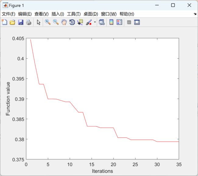
figure (1)
plot(bsof,'r'); xlabel('Iterations'); ylabel('Function value')
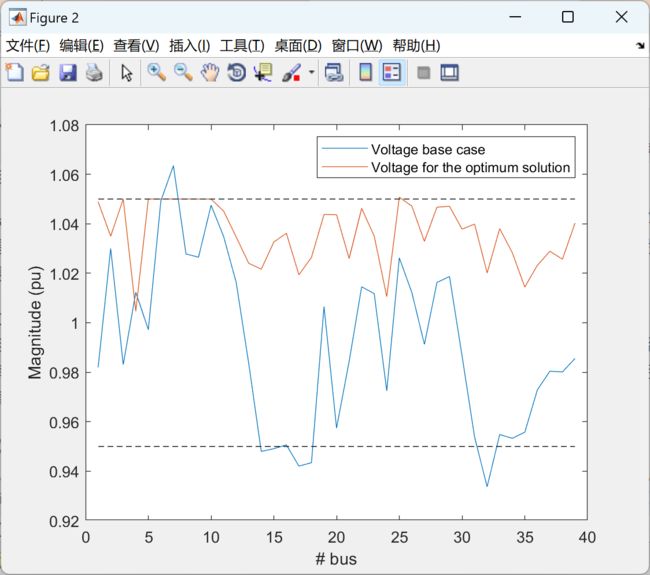
figure (2)
title('Voltage profile')
for k=1:n_nodos
Lim1(k)=0.95;
Lim2(k)=1.05;
end
plot(V_o); hold on; plot(Vs); hold on; plot(Lim1,'--k'); hold on; plot(Lim2,'--k'); xlabel('# bus'); ylabel('Magnitude (pu)')
legend('Voltage base case','Voltage for the optimum solution')
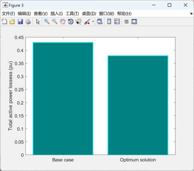
figure (3)
title('Active power lossess')
y=[Plosses,Pls];
c=categorical({'Base case','Optimum solution'});
bar(c,y,'FaceColor',[0 .5 .5],'EdgeColor',[0 .9 .9],'LineWidth',1.5)
ylabel('Total active power lossess (pu)')
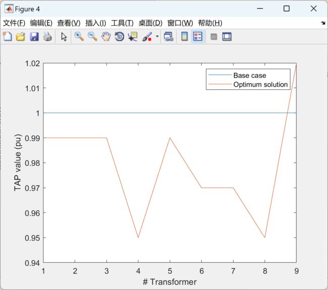
figure (4)
title('TAP values comparison')
plot(tap_o); hold on; plot(xitap(end,:)); xlabel('# Transformer'); ylabel('TAP value (pu)')
legend('Base case','Optimum solution')
3 参考文献
文章中一些内容引自网络,会注明出处或引用为参考文献,难免有未尽之处,如有不妥,请随时联系删除。
[1]李璇.基于遗传算法的电力系统最优潮流问题研究[D].华中科技大学,2007.
[2]尤金.基于Jaya算法的DG优化配置研究[D].天津大学,2018.
[3]蒋承刚,熊国江,帅茂杭.基于DE-Jaya混合优化算法的电力系统经济调度方法[J].传感器与微系统, 2023.