R语言:主成分分析PCA
文章目录
-
-
-
- 主成分分析
- 处理步骤
- 数据集
- code
-
-
主成分分析
主成分分析(或称主分量分析,principal component analysis)由皮尔逊(Pearson,1901)首先引入,后来被霍特林(Hotelling,1933)发展。
主成分分析是一种通过降维技术把多个变量化为少数几个主成分(即综合变量)的统计分析方法。这些主成分能够反映原始变量的绝大部分信息,它们通常表示为原始变量的某种线性组合。
- 主成分分析的一般目的是:
- 变量的降维;
- 主成分的解释。
处理步骤
-
将数据标准化(必需,不同量纲和大小的数据影响结果)
-
求样本的相关系数矩阵
R -
求
R的特征值以及特征向量 -
按主成分累计贡献率超过
80%来确定主成分的个数K,并写出主成分表达式(一般是80%,实际问题中70%多也可以接受) -
对分析结果做统计意义和实际意义的解释(往往是更难的)
数据集
内置的mtcars数据框包含有关32辆汽车的信息,包括它们的重量,燃油效率(以每加仑英里为单位),速度等。
数据来自1974年美国汽车趋势杂志,包括32辆汽车(1973-74款)的油耗和10个方面的汽车设计和性能。
> help("mtcars")

Motor Trend Car Road Tests
Description
The data was extracted from the 1974 Motor Trend US magazine, and comprises fuel consumption and 10 aspects of automobile design and performance for 32 automobiles (1973–74 models).

Usage
mtcars
Format
A data frame with 32 observations on 11 (numeric) variables.

[, 1]	mpg	Miles/(US) gallon
[, 2]	cyl	Number of cylinders
[, 3]	disp	Displacement (cu.in.)
[, 4]	hp	Gross horsepower
[, 5]	drat	Rear axle ratio
[, 6]	wt	Weight (1000 lbs)
[, 7]	qsec	1/4 mile time
[, 8]	vs	Engine (0 = V-shaped, 1 = straight)
[, 9]	am	Transmission (0 = automatic, 1 = manual)
[,10]	gear	Number of forward gears
[,11]	carb	Number of carburetors
Source
Henderson and Velleman (1981), Building multiple regression models interactively. Biometrics, 37, 391–411.

Examples
require(graphics)
pairs(mtcars, main = "mtcars data", gap = 1/4)
coplot(mpg ~ disp | as.factor(cyl), data = mtcars,
       panel = panel.smooth, rows = 1)
## possibly more meaningful, e.g., for summary() or bivariate plots:
mtcars2 <- within(mtcars, {
   vs <- factor(vs, labels = c("V", "S"))
   am <- factor(am, labels = c("automatic", "manual"))
   cyl  <- ordered(cyl)
   gear <- ordered(gear)
   carb <- ordered(carb)
})
summary(mtcars2)
code
- 计算相关系数矩阵
#计算相关系数
R<-cor(mtcars)
R

           mpg        cyl       disp         hp        drat         wt
mpg   1.0000000 -0.8521620 -0.8475514 -0.7761684  0.68117191 -0.8676594
cyl  -0.8521620  1.0000000  0.9020329  0.8324475 -0.69993811  0.7824958
disp -0.8475514  0.9020329  1.0000000  0.7909486 -0.71021393  0.8879799
hp   -0.7761684  0.8324475  0.7909486  1.0000000 -0.44875912  0.6587479
drat  0.6811719 -0.6999381 -0.7102139 -0.4487591  1.00000000 -0.7124406
wt   -0.8676594  0.7824958  0.8879799  0.6587479 -0.71244065  1.0000000
qsec  0.4186840 -0.5912421 -0.4336979 -0.7082234  0.09120476 -0.1747159
vs    0.6640389 -0.8108118 -0.7104159 -0.7230967  0.44027846 -0.5549157
am    0.5998324 -0.5226070 -0.5912270 -0.2432043  0.71271113 -0.6924953
gear  0.4802848 -0.4926866 -0.5555692 -0.1257043  0.69961013 -0.5832870
carb -0.5509251  0.5269883  0.3949769  0.7498125 -0.09078980  0.4276059
            qsec         vs          am       gear        carb
mpg   0.41868403  0.6640389  0.59983243  0.4802848 -0.55092507
cyl  -0.59124207 -0.8108118 -0.52260705 -0.4926866  0.52698829
disp -0.43369788 -0.7104159 -0.59122704 -0.5555692  0.39497686
hp   -0.70822339 -0.7230967 -0.24320426 -0.1257043  0.74981247
drat  0.09120476  0.4402785  0.71271113  0.6996101 -0.09078980
wt   -0.17471588 -0.5549157 -0.69249526 -0.5832870  0.42760594
qsec  1.00000000  0.7445354 -0.22986086 -0.2126822 -0.65624923
vs    0.74453544  1.0000000  0.16834512  0.2060233 -0.56960714
am   -0.22986086  0.1683451  1.00000000  0.7940588  0.05753435
gear -0.21268223  0.2060233  0.79405876  1.0000000  0.27407284
carb -0.65624923 -0.5696071  0.05753435  0.2740728  1.00000000
- 计算特征值
#计算特征值
lambda<-princomp(R)
lambda

Call:
princomp(x = R)

Standard deviations:
     Comp.1      Comp.2      Comp.3      Comp.4
1.992444019 0.762563719 0.164481730 0.079889308
     Comp.5      Comp.6      Comp.7      Comp.8
0.065557778 0.052541093 0.040670837 0.024829720
     Comp.9     Comp.10     Comp.11
0.022722621 0.006649006 0.000000000

 11  variables and  11 observations.
- 计算标准差,贡献率,累计贡献率
Standard deviation:标准差
Proportion of Variance:方差贡献率
Cumulative Proportion:累积贡献率
Loadings:载荷矩阵
#计算标准差,贡献率,累计贡献率
summary(lambda,loadings=TRUE)

Importance of components:
                          Comp.1    Comp.2      Comp.3      Comp.4
Standard deviation     1.9924440 0.7625637 0.164481730 0.079889308
Proportion of Variance 0.8640097 0.1265606 0.005888188 0.001389069
Cumulative Proportion  0.8640097 0.9905703 0.996458532 0.997847601
                             Comp.5       Comp.6       Comp.7
Standard deviation     0.0655577780 0.0525410926 0.0406708369
Proportion of Variance 0.0009353945 0.0006008203 0.0003600084
Cumulative Proportion  0.9987829955 0.9993838158 0.9997438241
                             Comp.8       Comp.9      Comp.10 Comp.11
Standard deviation     0.0248297195 0.0227226207 6.649006e-03       0
Proportion of Variance 0.0001341807 0.0001123733 9.621877e-06       0
Cumulative Proportion  0.9998780048 0.9999903781 1.000000e+00       1

Loadings:
     Comp.1 Comp.2 Comp.3 Comp.4 Comp.5 Comp.6 Comp.7 Comp.8 Comp.9
mpg   0.363         0.290                0.274  0.242  0.514  0.524
cyl  -0.374         0.192        -0.136  0.277        -0.282 -0.178
disp -0.368         0.158 -0.129        -0.451  0.232  0.109  0.285
hp   -0.330  0.238         0.155 -0.441 -0.193         0.647 -0.290
drat  0.295  0.263 -0.117 -0.856 -0.268
wt   -0.346 -0.162 -0.278 -0.207  0.350 -0.335                0.413
qsec  0.200 -0.483 -0.344         0.344                0.361 -0.438
vs    0.306 -0.252 -0.383  0.278 -0.570 -0.234 -0.249 -0.192  0.289
am    0.235  0.431  0.247  0.125  0.322 -0.427 -0.575
gear  0.208  0.450 -0.304  0.277  0.129 -0.247  0.657 -0.200 -0.119
carb -0.213  0.396 -0.580         0.151  0.438 -0.248  0.124  0.252
     Comp.10 Comp.11
mpg   0.132   0.289
cyl   0.164   0.766
disp -0.656   0.182
hp    0.254
drat          0.132
wt    0.569
qsec -0.171   0.363
vs            0.236
am            0.249
gear          0.136
carb -0.318
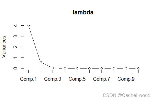
由上表结果可知,一个主成分y1的方差贡献率已经达到86.4%,前两个主成分的累积方差贡献率达到99.06%,已经完全可以解释总方差。
- 画出碎石图
#画出碎石图
screeplot(lambda,type = "lines")
-
写出对应主成分表达式
通过载荷矩阵loadings写出对应的主成分 -
画出载荷散点图
#提取主成分载荷矩阵
load<-loadings(student.pr)
#用载荷前两列做散点图
plot(load[,1:2],xlim=c(-0.9,0.9),ylim=c(-0.9,0.9))
#标记序号
text(load[,1],load[,2],adj=c(0.9,-0.9))
#划分象限
abline(h=0);abline(v=0)
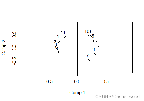
从载荷散点图可以看出,各变量与两个主成分之间的关系并不明显,使用主成分分析的效果并不够好。
虽然在方差贡献率上主成分分析PCA表现良好,但是解释性(往往是最重要的)比较差。