随机规划——报童模型
参考文献:github上一个老师的代码。
理论知识
基于CVaR准则的报童模型
令n表示 len(demand.values),其中demand.values表示需求分布中的每一个需求值。
for i=1,2,3,…,n
当需求为 d e m a n d [ i ] demand[i] demand[i]时,
定义利润函数为 p r o f i t [ i ] profit[i] profit[i],
定义损失函数为 l o s s [ i ] = − p r o f i t [ i ] loss[i]=-profit[i] loss[i]=−profit[i] (在程序中没有),
optimizer.py中min_conditional_value_at_risk_solution这段程序的决策变量有: p r o f i t [ i ] , s a l e s [ i ] , o r d e r , e x c e s s [ i ] , t profit[i], sales[i], order,excess[i],t profit[i],sales[i],order,excess[i],t,
其中, s a l e s [ i ] sales[i] sales[i]表示销售量;
定义决策变量 e x c e s s [ i ] = ( l o s s [ i ] − t ) + excess[i]=(loss[i]-t)^+ excess[i]=(loss[i]−t)+,那么产生约束 e x c e s s [ i ] ≥ − p r o f i t [ i ] − t excess[i]\geq -profit[i]-t excess[i]≥−profit[i]−t;
销售量一定不会超过订货量,那么产生约束 o r d e r − s a l e s [ i ] > = 0 ; order-sales[i]>=0; order−sales[i]>=0;
销售量一定不会超过需求量,那么产生约束 s a l e s [ i ] < = d e m a n d [ i ] sales[i]<=demand[i] sales[i]<=demand[i],
根据利润的计算公式,产生等式约束 p r o f i t [ i ] = s a l e s [ i ] ∗ u n i t S a l e s P r i c e − o r d e r ∗ u n i t C o s t profit[i]=sales[i]*unitSalesPrice-order*unitCost profit[i]=sales[i]∗unitSalesPrice−order∗unitCost;
根据CVaR准则,在置信水平 α \alpha α下,零售商预期损失的条件风险值 α − C V a R \alpha-CVaR α−CVaR为
C V a R α ( C ( o r d e r ) ) = E [ C ( o r d e r ) ∣ C ( o r d e r ) > = V a R α ( C ( o r d e r ) ) ] CVaR_\alpha(C(order))=E[C(order)|C(order)>=VaR_\alpha(C(order))] CVaRα(C(order))=E[C(order)∣C(order)>=VaRα(C(order))],
其中, V a R α ( C ( o r d e r ) ) = i n f { k ∈ R ∣ P r o b ( C ( o r d e r ) < = k ) > = α } VaR_\alpha(C(order))=inf\{k\in R|Prob(C(order)<=k)>=\alpha\} VaRα(C(order))=inf{k∈R∣Prob(C(order)<=k)>=α}
0 < = α < = 1 0<=\alpha<=1 0<=α<=1
V a R α ( C ( o r d e r ) ) VaR_\alpha(C(order)) VaRα(C(order))表示零售商的在险价值;
α \alpha α为置信水平,表示损失不超过VaR的概率下界。
对于风险厌恶型零售商,使得 C V a R α ( C ( o r d e r ) ) CVaR_\alpha(C(order)) CVaRα(C(order))最小的订货量表示零售商的最优订货量,
即 m i n q > = 0 C V a R α ( C ( o r d e r ) ) min_{q>=0}CVaR_\alpha(C(order)) minq>=0CVaRα(C(order)).
目标函数是最小化如下表达式
t + ∑ i = 1 n e x c e s s [ i ] ∗ P r o b [ i ] / ( 1 − α ) t+\sum_{i=1}^nexcess[i]*Prob[i]/(1-\alpha) t+∑i=1nexcess[i]∗Prob[i]/(1−α)
(注:怎么理解这个表达式呢?可以把excess[i]=(loss[i]-t)^+带入到上式,得到成本函数的加权平均,也就是 C V a R α ( C ( o r d e r ) ) = E [ C ( o r d e r ) ∣ C ( o r d e r ) > = V a R α ( C ( o r d e r ) ) ] CVaR_\alpha(C(order))=E[C(order)|C(order)>=VaR_\alpha(C(order))] CVaRα(C(order))=E[C(order)∣C(order)>=VaRα(C(order))])
基于VaR准则的报童模型
VaR: value_at_risk;
这里使用随机线性规划解报童模型,目标函数是 m i n V a R α ( l o s s ) min VaR_\alpha(loss) minVaRα(loss);
引入01决策变量,将问题转成MIP,从而能够计算分位数。
为了计算VaR,这里使用下述技巧
L [ D ] L[D] L[D]表示损失,依赖于需求量D;
V a R α ( L [ D ] ) : = m i n { v ∣ P r ( L [ D ] < = v ) > = a } VaR_\alpha(L[D]):=min\{v|Pr(L[D]<=v)>=a\} VaRα(L[D]):=min{v∣Pr(L[D]<=v)>=a}
其中,概率可以表示成加和的形式,如下
P r ( L [ D ] < = v ) = E { I ( L [ D ] < = v ) } = ∑ d P r ( D = d ) ∗ I ( L [ D ] < = v ) Pr(L[D]<=v)=E\{ I(L[D]<=v) \}=\sum_dPr(D=d)*I(L[D]<=v) Pr(L[D]<=v)=E{I(L[D]<=v)}=∑dPr(D=d)∗I(L[D]<=v);
引入二进制变量 i s R i s k L o w e r T h a n V a R [ d ] : = I ( L [ d ] < = V a R ) isRiskLowerThanVaR[d]:=I(L[d]<=VaR) isRiskLowerThanVaR[d]:=I(L[d]<=VaR)
也就是说,如果 L [ d ] < = V a R L[d]<=VaR L[d]<=VaR,那么 i s R i s k L o w e r T h a n V a R [ d ] = 1 isRiskLowerThanVaR[d]=1 isRiskLowerThanVaR[d]=1,否则 i s R i s k L o w e r T h a n V a R [ d ] = 0 isRiskLowerThanVaR[d]=0 isRiskLowerThanVaR[d]=0.
下面将这个指示性约束线性化,如下
L ∗ ( 1 − i s R i s k L o w e r T h a n V a R [ d ] ) < = V a R − L [ d ] < = U ∗ i s R i s k L o w e r T h a n V a R [ d ] ) L*(1-isRiskLowerThanVaR[d])<=VaR-L[d]<=U*isRiskLowerThanVaR[d]) L∗(1−isRiskLowerThanVaR[d])<=VaR−L[d]<=U∗isRiskLowerThanVaR[d])
其中,L,U分别是 V a R − L [ d ] VaR-L[d] VaR−L[d]的下界、上界。
所以,这个约束 P r ( L [ D ] < = v ) > = a Pr(L[D]<=v)>=a Pr(L[D]<=v)>=a可以写成 ∑ d P r ( D = d ) ∗ i s R i s k L o w e r T h a n V a R [ d ] > = a \sum_dPr(D=d)*isRiskLowerThanVaR[d]>=a ∑dPr(D=d)∗isRiskLowerThanVaR[d]>=a.
Python代码
简介
由三个模块构成,分别是optimizer模块、simulator模块、main模块。
- optimizer.py定义了四种版本的报童模型、Demand类(由离散随机分布、抽样函数所构成)
- simulator.py定义了绘制数组的概率分布图、累计概率分布图等,计算利润的函数;
- main.py调用了optimizer.py和simulator.py两个模块的函数和类,具体地,定义了一个枚举类ProblemInstance,枚举了四种版本的报童模型。另外,这个枚举类定义了方法
.solve,当检查到对象是某个枚举元素(某个版本的报童模型)时,调用optimizer.py中对应的函数,从而给出最优订货量。 - 顺序:先布置optimizer模块,再simulator模块,最后是 main模块。
这套代码一共实现了四个版本的报童模型,他们的目标函数不同。
分别是
- 用解析解, m a x E [ p r o f i t s ] max E[profits] maxE[profits]
- 用线性规划解, m a x E [ p r o f i t s ] max E[profits] maxE[profits]
- 用线性规划解, m i n V a R α [ − p r o f i t s ] min VaR_\alpha[-profits] minVaRα[−profits]
- 用线性规划解, m i n C V a R α [ − p r o f i t s ] min CVaR_\alpha[-profits] minCVaRα[−profits]
在模块optimizer.py,对于每一个版本的报童模型搭建与求解,都会新建一个函数。这四个函数分别为max_expected_profit_analytic_solution,
max_expected_profit_solution,
min_value_at_risk_solution,
min_conditional_value_at_risk_solution。
源代码
optimizer.py
# -*- coding: utf-8 -*-

"""
Several implementations of the news vendor problem.
---------
In this problem, a paperboy has to buy N newspapers at cost C that he will sell the next day at price P.
The next-day demand for newspapers is random, and the paperboy needs to carefully build his inventory so
as to maximize his profits while hedging against loss.
"""

import math
from functools import cached_property
from logging import getLogger
from typing import List

import gurobipy as gp
import numpy as np
import scipy
# from gurobipy import GRB
# import gurobipy.GRB as GRB
from gurobipy.gurobipy import GRB

logger = getLogger(__name__)


class Demand:

    EPS = 1e-6

    def __init__(self, rv: scipy.stats.rv_discrete, seed: int = 42) -> None:
        self.rv = rv # customized weight
        self.rv.random_state = np.random.RandomState(seed=seed)

    @cached_property
    def values(self) -> List[int]:
        _min = self.rv.ppf(self.EPS)
        _max = self.rv.ppf(1 - self.EPS)
        return [*range(math.floor(_min), math.ceil(_max) + 1)]

    def samples(self, sample_size: int) -> np.ndarray:
        return self.rv.rvs(sample_size)

# the following 4 models all return order_quantiy
def max_expected_profit_analytic_solution(
    demand: Demand,# Demand class
    unit_cost: float,
    unit_sales_price: float,
) -> float:
    """
    Analytically computes the solution (number of orders) of the news vendor problem - with max E[profit] objective
    order* = F^(-1)[(p - c) / p]
    """
    return demand.rv.ppf((unit_sales_price - unit_cost) / unit_sales_price) # return the corresponding demand_value


def max_expected_profit_solution(
    demand: Demand,
    unit_cost: float,
    unit_sales_price: float,
) -> float:
    """
    Solves the news vendor problem using stochastic linear programming
    with max E[profits] objective: E[profits] = ∑ proba[Ω] * profits[Ω]
    """

    model = gp.Model("news_vendor_expectation")

    order = model.addVar(lb=0, name="order")
    sales = model.addVars(demand.values, lb=0, ub=max(demand.values), name="sales")# all the possible demand_value

    model.addConstrs(order - sales[d] >= 0 for d in demand.values)
    model.addConstrs(sales[d] <= d for d in demand.values)# 销量 必然不大于 需求量

    model.setObjective(
        gp.quicksum(
            (sales[d] * unit_sales_price - order * unit_cost) * demand.rv.pmf(d)
            for d in demand.values
        ),
        GRB.MAXIMIZE,
    )

    model.optimize()

    return order.X


def min_conditional_value_at_risk_solution(
    demand: Demand,
    unit_cost: float,
    unit_sales_price: float,
    alpha: float,
) -> float:
    """
    Solves the news vendor problem using stochastic linear programming
    with min CVaR_a[loss] objective.
    We use the following trick to compute CVaR: CVaR_a[loss[D]] = min t + E[|loss[D] - t|^+] / (1 - a)
    """

    model = gp.Model("news_vendor_CVaR")

    order = model.addVar(lb=0, name="order")
    sales = model.addVars(demand.values, lb=0, ub=max(demand.values), name="sales") # demand.values is index of decision_vars sales

    t = model.addVar(lb=-GRB.INFINITY, name="t")# value_at_risk
    # excess := |loss[Ω] - t|+
    excess = model.addVars(demand.values, lb=0, name="excess")
    # profit := -loss
    profit = model.addVars(demand.values, lb=-GRB.INFINITY, name="profit")

    model.addConstrs(order - sales[d] >= 0 for d in demand.values) # we don't consider lost sales
    model.addConstrs(sales[d] <= d for d in demand.values)
    model.addConstrs(
        profit[d] == sales[d] * unit_sales_price - order * unit_cost
        for d in demand.values
    )

    model.addConstrs(excess[d] >= -profit[d] - t for d in demand.values)

    # fmt: off # ?? what fmt
    model.setObjective(
        t + gp.quicksum(
            (excess[d] / (1 - alpha)) * demand.rv.pmf(d) for d in demand.values
        ),
        GRB.MINIMIZE,
    )
    # fmt: on

    model.optimize()

    return order.X


def min_value_at_risk_solution(
    demand: Demand,
    unit_cost: float,
    unit_sales_price: float,
    alpha: float,
) -> float: # return order_quantity
    """
    Solves the news vendor problem using stochastic linear programming
    with min VaR_a[loss] objective.
    We need to introduce binary variables (therefore the problem becomes a MIP) in order
    to compute quantiles. The formulation is quite poor as it relies on large big-M tricks.
    This seems coherent with the remark from https://www.youtube.com/watch?v=Jb4a8T5qyVQ
    > "it becomes a "bad" MIP, need to track every-scenario"

    To compute the VaR we use the following trick:
    > VaR_a[L[D]] := min { v | P(L[D] ≤ v) ≥ a } (with L[D] being the loss, that depends on the demand r.v.)
    > We have P(L[D] ≤ v) = E[ indicator(L[D] ≤ v) ] = ∑_{d} P(D=d) * indicator(L[d] ≤ v)
    > The role of the introduced binary variables is to compute is_risk_lower_than_VaR[d] := indicator(L[d] ≤ VaR)
    """

    model = gp.Model("news_vendor_VaR")

    order = model.addVar(lb=0, name="order")
    sales = model.addVars(demand.values, lb=0, ub=max(demand.values), name="sales")
    value_at_risk = model.addVar(name="value_at_risk", lb=-1e6, ub=1e6)
    risk = model.addVars(demand.values, name="risk", lb=-1e6, ub=1e6)  # risk := loss , reference to the CVaR case
    # is_risk_lower_than_VaR[d] := 1 if value_at_risk >= risk[d], else 0
    is_risk_lower_than_VaR = model.addVars(
        demand.values, vtype=GRB.BINARY, name="is_risk_lower_than_VaR"
    )

    model.addConstrs(order - sales[d] >= 0 for d in demand.values)
    model.addConstrs(sales[d] <= d for d in demand.values)

    model.addConstrs(
        risk[d] == order * unit_cost - sales[d] * unit_sales_price # net cost
        for d in demand.values
    )

    # We use a big-M trick here to linearize the constraint `is_risk_lower_than_VaR[d] := 1 if value_at_risk >= risk[d], else 0`
    # L * (1 - is_risk_lower_than_VaR[d]) <= value_at_risk - risk[d] <= U * count_value_at_risk[d]
    # where L and U are lower and upper bounds for `value_at_risk - risk[d]`
    # TODO: remove hardcoded variables
    L, U = -1e6, +1e6
    model.addConstrs(
        L * (1 - is_risk_lower_than_VaR[d]) <= value_at_risk - risk[d]
        for d in demand.values
    )
    model.addConstrs(
        value_at_risk - risk[d] <= U * (is_risk_lower_than_VaR[d])
        for d in demand.values
    )

    # VaR definition as a alpha quantile
    model.addConstr(
        gp.quicksum(is_risk_lower_than_VaR[d] * demand.rv.pmf(d) for d in demand.values)
        >= alpha
    )

    model.setObjective(value_at_risk, GRB.MINIMIZE)

    model.optimize()

    return order.X
simulator.py
# -*- coding: utf-8 -*-
from logging import getLogger
from typing import Iterable, Optional, Tuple

import matplotlib
import matplotlib.pyplot as plt
import numpy as np

# from stochastic_optimization.news_vendor.optimizer import Demand
from optimizer import Demand

logger = getLogger(__name__)


def simulate_profits(
    demand: Demand,
    unit_cost: float,
    unit_sales_price: float,
    order: float,
    sample_size: int = 1000,
) -> np.ndarray:
    """
    Simulates a news vendor profits for a given random demand, unit cost & price, and a chosen order
    """
    demand_samples = demand.samples(sample_size=sample_size)
    sales = np.minimum(order, demand_samples) # actual sales, ndarray, !! use np.minimum, instead of np.min
    profits = sales * unit_sales_price - order * unit_cost
    return profits # ndarray


def plot_distribution(
    samples: Iterable[float],
    title: Optional[str] = None,
    outstanding_points: Iterable[Tuple[str, float]] = (),
) -> None:
    """
    Helper function to plot the distribution and cumulative distribution of a series of samples
    from a random variable
    """

    ax1 = plt.subplot()
    ax2 = ax1.twinx()
    ax1.hist(samples, density=True, label="Distribution", color="coral")
    ax2.hist(
        samples,
        density=True,
        histtype="step",
        cumulative=True,
        label="Cumulative distribution",
        color="darkred",
    )

    if title:
        plt.title(title)

    colors = matplotlib.cm.cool(np.linspace(0, 1, len(outstanding_points))) # ready for vertivcal_line of outstanding_points
    for i, outstanding_point in enumerate(outstanding_points):
        # outstanding_points's usage like ("average_profit",np.mean(profits))
        ax2.vlines(
            x=outstanding_point[1],# float, np.mean(profits)
            ymin=0,
            ymax=1,
            label=outstanding_point[0],# string, "average_profit"
            color=colors[i],
        )

    h1, l1 = ax1.get_legend_handles_labels()
    h2, l2 = ax2.get_legend_handles_labels()
    ax1.legend(h1 + h2, l1 + l2, loc=2)

    plt.show()
main.py
# -*- coding: utf-8 -*-
"""
Main entrypoint to the news vendor problem implementation.
Use this script to run an instance of the problem,
get a solution and plot the profits distribution to visualize
if you're hedging against risk.
"""
from enum import Enum
from typing import List, Optional

import numpy as np
import scipy

from stochastic_optimization.news_vendor.optimizer import (
    Demand,
    max_expected_profit_analytic_solution,
    max_expected_profit_solution,
    min_conditional_value_at_risk_solution,
    min_value_at_risk_solution,
)
from stochastic_optimization.news_vendor.simulator import (
    plot_distribution,
    simulate_profits,
)


def get_scipy_discrete_distributions() -> List[str]:
    """Returns the list of scipy discrete distributions supported by the model"""
    discrete_distributions: List[str] = []
    for distribution_name in dir(scipy.stats):
        if isinstance(getattr(scipy.stats, distribution_name), scipy.stats.rv_discrete):
            discrete_distributions.append(distribution_name)
    return discrete_distributions


class ProblemInstance(Enum):
    expected_profit_analytic = "expected_profit_analytic"
    expected_profit_lp = "expected_profit_lp"
    VaR = "VaR"
    CVaR = "CVaR"

    @property
    def solve(self) -> "function":
        if self == self.expected_profit_analytic:
            return max_expected_profit_analytic_solution

        if self == self.expected_profit_lp:
            return max_expected_profit_solution

        if self == self.VaR:
            return min_value_at_risk_solution

        if self == self.CVaR:
            return min_conditional_value_at_risk_solution

        raise NotImplementedError()

    @property
    def is_alpha_expected(self) -> bool:
        return self in [self.VaR, self.CVaR]


def solve(
    problem: ProblemInstance,
    demand: Demand,
    unit_cost: float,
    unit_sales_price: float,
    alpha: Optional[float] = None,
    sample_size: int = 1000,
) -> None:

    plot_distribution(
        demand.samples(sample_size),
        title="Demand",
        outstanding_points=[("Average demand", demand.rv.mean())],
    )

    kwargs = {}
    if problem.is_alpha_expected:
        kwargs["alpha"] = alpha if alpha is not None else 0.75

    order = problem.solve(demand, unit_cost, unit_sales_price, **kwargs) # call one of four methods, like max_expected_profit_analytics_solution, lp, min_var_solution and so on

    profits = simulate_profits(
        demand,
        unit_cost,
        unit_sales_price,
        order,
        sample_size,
    )

    plot_distribution(
        profits,
        title=f"Profits - {problem.name}",
        outstanding_points=[
            ("Null profit", 0),
            ("Expected profit", np.mean(profits)),
            ("Min profit", np.min(profits)),
        ],
    )
源代码学习启示
注意,
- 枚举类
ProblemInstance的定义与使用; - 定义类的各个方法,使用
property等装饰器
数值实验
随机优化的目标是如何shift distribution of your economic objective。(没看懂,硬翻译就是这样,,,) 将要赚取的最大利润是什么?坏事发生的机率如何?
- 最大化期望利润
好的健全性检查(good sanity check):解线性规划模型得到的解和推导公式得到的解析解,会得到同样的结果、相同的利润分布。 - 实验参数的设置
假设低利润场景, 购买成本为1,零售价格为1.1,假设需求数据服从分布Poisson(mu=100)。
在main.py里面,写一个主函数,如下,从而得到下述实验结果
if __name__=="__main__":
    print(get_scipy_discrete_distributions())
    Problem=ProblemInstance.VaR # .CVaR, .expected_profit_analytic, .expected_profit_lp
    solve(Problem,Demand(scipy.stats.poisson(100)),1,1.1,.8)
    # params: Problem,Demand,unit_cost,unit_sales_price, alpha
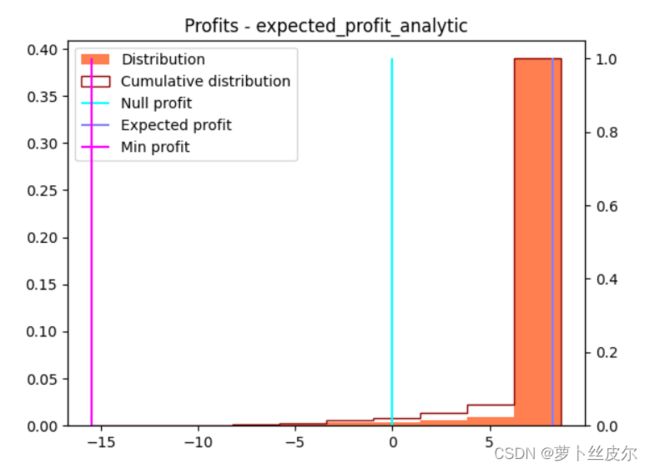
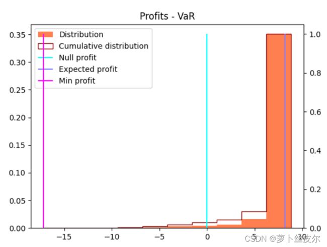
天蓝色的竖线(Null Profit)表示不盈利;
紫红色的竖线(Min Profit)表示 盈利最小值;
蓝紫色的竖线(Expect Profit)表示 盈利均值。
绿色柱子表示profits这个数组的分布情况。

注:下面图的题目中 以Profit打头的,表示在最优订货量的情况下,利润的分布。如,Profit_CVaR表示第四版本的报童模型(目标是最小化 C V a R α ( L o s s ( D ) ) CVaR_\alpha(Loss(D)) CVaRα(Loss(D)))
最小化 C V a R α CVaR_\alpha CVaRα会把利润(或损失)分布压缩到一个小范围,也就是说,我们以牺牲极好情况下的高利润为代价,来规避坏情况的出现。

上图是α=0.85的利润分布([-8,8]),下图是α=0.95的利润分布([-4,8])。通过比较可以看到,α越大,利润的分布范围越小。

再看”用推导公式得到的最优订货量(解析解)下,零售商的利润分布“,如下图,分布范围是[-15,5]。

- 最小化 V a R α VaR_\alpha VaRα会推着利润分布向右,挤成更小的取值范围。同样地,以牺牲极大利润为代价,规避极差情况的发生。有点惊人的是,它也能改进期望利润。但,好情况下的最大利润值降低了,这是意料中的。

上图是 α = 0.85 \alpha=0.85 α=0.85,下图是 α = 0.95 \alpha=0.95 α=0.95,可以看到蓝紫色竖线向x轴右端移动了,也就是说,随着 α \alpha α的增大,利润均值增大了。
为了能够对比出结果,下面是用解析解给出利润分布图