KITTI数据集简介

本文节选自这里

Kitti data format

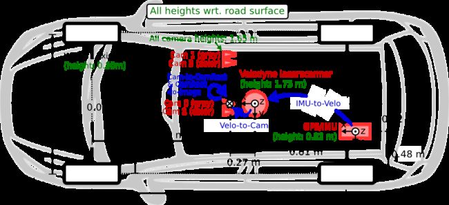
Kitti data collection platform link:

The sensor coordinate is shown in the following figure:

Kitt dataset folders are

• {training,testing}/image_2/id.png
• {training,testing}/image_3/id.png
• {training,testing}/label_2/id.txt
• {training,testing}/velodyne/id.bin
• {training,testing}/calib/id.txt

The coordinate system of the following sensors:

• Camera: x = right, y = down, z = forward
• Velodyne: x = forward, y = left, z = up
• GPS/IMU: x = forward, y = left, z = up

The cameras are mounted approximately level with the ground plane. The camera images are cropped to a size of 1382 x 512 pixels using libdc’s format 7 mode. After rectification, the images get slightly smaller. The cameras are triggered at 10 frames per second by the laser scanner (when facing forward) with shutter time adjusted dynamically (maximum shutter time: 2 ms).

Each point cloud is an unordered set of returned lidar points. The data format of each returned lidar point is a 4-tuple formed by its coordinate with respect to the lidar coordinate frame as well as its intensity ρ. In the KITTI dataset, ρ is a normalized value between 0 and 1, and it depends on the characteristics of the surface the lidar beam reflecting from. The KITTI dataset represents the returned lidar points using their cartesian coordinates in the lidar coordinate frame as well as their intensities as follows: (x, y, z, ρ). Lidar point cloud is stored in fileid.bin: 2D array with shape [num_points, 4] Each point encodes XYZ + reflectance. The laser scanner spins at 10 frames per second, capturing approximately 100k points per cycle. The vertical resolution of the laser scanner is 64. Each scene point cloud in the KITTI dataset has on average about 100K points.

Object instance is stored in fileid_label.txt : For each row, the annotation of each object is provided with 15 columns representing certain metadata and 3D box properties in camera coordinates: type | truncation | visibility | observation angle | xmin | ymin |xmax | ymax | height | width | length | tx | ty | tz | roty
Some instances typeare marked as ‘DontCare’, indicating they are not labelled. The box dimensions are simply its width, length and height (w, l, h) and the coordinates of the center of the box (x, y, z).

In Kitti Devkit, the full definition is
. Kitti original paper

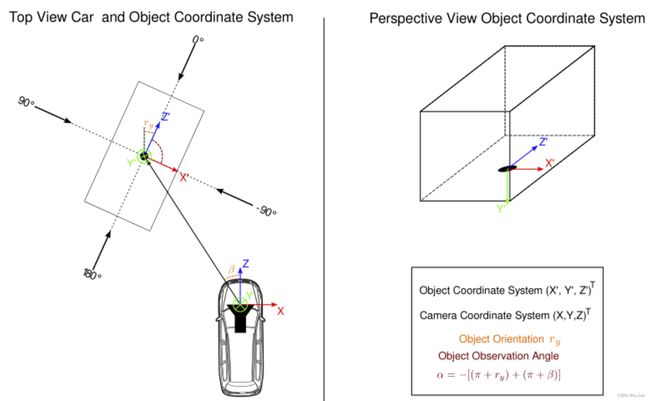
The difference between rotation_y (Rotation ry around Y-axis in camera coordinates [-pi…pi]) and alpha (Observation angle of object, ranging [-pi…pi]) is, that rotation_y is directly given in camera coordinates, while alpha also considers the vector from the camera center to the object center, to compute the relative orientation of the object with respect to the camera.

• For example, a car which is facing along the X-axis of the camera coordinate system corresponds to rotation_y=0, no matter where it is located in the X/Z plane (bird’s eye view)
• alpha is zero when this object is located along the Z-axis (front) of the camera.
  

Calibration

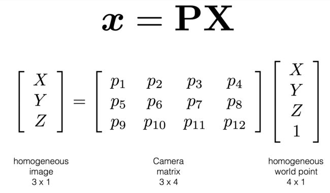
The “calib” folder contains all calibration parameters as shown in the following image. All calibration files are similar, except the first 000000.txt file. The calibration parameters are stored in row-major order. It contains the 3x4 projection matrix parameters which describe the mapping of 3D points in the world to 2D points in an image.

All matrices are stored row-major, i.e., the first values correspond to the first row. The calibration is done with cam0 as the reference sensor. The laser scanner is registered with respect to the reference camera coordinate system. Rectification R_ref2rect has also been considered during calibration to correct for planar alignment between cameras. The coordinates in the camera coordinate system can be projected in the image by using the 3x4 projection matrix in the calib folder (the left color camera (camera2) should use P2).

• P_rect[i] (P0, P1, P2, P3): projective transformation from rectified reference camera frame to cam[i]
• R0_rect : rotation to account for rectification for points in the reference camera. R0_rect contains a 3x3 matrix which you need to extend to a 4x4 matrix by adding a 1 as the bottom-right element and 0’s elsewhere
• Tr_velo_to_cam is 3x4 matrix (R|t): euclidean transformation from lidar to reference camera cam0. You need to extend to a 4x4 matrix in the same way

From the annotation, we are given the location of the box (t), the yaw angle ® of the box in camera coordinates (save to assume no pitch and roll) and the dimensions: height (h), width (w) and length (l). Note that 3D boxes of objects are annotated in camera coordinate.

Project Lidar to Camera

Projection from lidar to camera 2 (project_velo_to_cam2): the following transformations are considered: proj_mat = P_rect2cam2 @ R_ref2rect @ P_velo2cam_ref. The conversion process is shown in the following figure.

3d XYZ in .txt are in rect camera coord. 2d box xy are in image2 coord. Points in .bin are in Velodyne coord. project_velo_to_rect contains three main steps:

1. Velodyne points convert to reference camera (cam0) coordinate: x_ref = Tr_velo_to_cam * x_velo, where x_velo is the lidar points, Tr_velo_to_cam (in calibration file) is the euclidean transformation from lidar to reference camera cam0.
2. Reference camera (cam0) coordinate to the recitified camera coordinate: x_rect = R0_rect * x_ref, where R0_rect is the rotation to account for rectification for points in the reference camera.
3. Project points in the rectified camera coordinate to the camera 2 coordinate: y_image2 = P^2_rect * x_rect = P^2_rect * R0_rect * Tr_velo_to_cam * x_velo, where P^2_rect is the projective transformation from rectified reference camera frame to cam2.

Based on the function “show_lidar_on_image–>call calib.project_velo_to_rect”, the velodyne points can be mapped to camera coordinate. “calib” is the instance of class Calibration

Code imgfov_pc_rect = calib.project_velo_to_rect(imgfov_pc_velo) contains two steps: 1) project_velo_to_ref via V2C (Tr_velo_to_cam); 2) project_ref_to_rect (via R0_rect). It finally returens imgfov_pc_rect, where imgfov_pc_rect[i, 2] is the depth, imgfov_pts_2d[i, 0] and imgfov_pts_2d[i, 1] are image width and height. Note: there is no projection (P^2_rect), that means the data in camera coordinate is still in 3D (with depth).

The following code can draw depth on mage:

img_lidar = show_lidar_on_image(pc_velo[:, :3], img, calib, img_width, img_height)
img_lidar = cv2.cvtColor(img_lidar, cv2.COLOR_BGR2RGB)

fig_lidar = plt.figure(figsize=(14, 7))
ax_lidar = fig_lidar.subplots()
ax_lidar.imshow(img_lidar)
plt.show()

Show 3D/2D box on image

The following code can draw 2D and 3D box on image:

img_bbox2d, img_bbox3d = show_image_with_boxes(img, objects, calib)

img_bbox2d = cv2.cvtColor(img_bbox2d, cv2.COLOR_BGR2RGB)
fig_bbox2d = plt.figure(figsize=(14, 7))
ax_bbox2d = fig_bbox2d.subplots()
ax_bbox2d.imshow(img_bbox2d)
plt.show()

img_bbox3d = cv2.cvtColor(img_bbox3d, cv2.COLOR_BGR2RGB)
fig_bbox3d = plt.figure(figsize=(14, 7))
ax_bbox3d = fig_bbox3d.subplots()
ax_bbox3d.imshow(img_bbox3d)
plt.show()

[show_image_with_boxes] contains the following major code (utils is Kitti.kitti_util)

box3d_pts_2d, _ = utils.compute_box_3d(obj, calib.P)
img2 = utils.draw_projected_box3d(img2, box3d_pts_2d)

“compute_box_3d” calculate corners_3d (8 corner points) based on the 3D bounding box (l,w,h), apply the rotation (ry), then add the translation (t). This calculation does not change the coordinate system (camera coordinate), only get the 8 corner points from the annotation (l,w,h, ry, and location t).

2D projections are obtained from

corners_2d = project_to_image(np.transpose(corners_3d), P)" 

def project_to_image(pts_3d, P):
    n = pts_3d.shape[0]
    pts_3d_extend = np.hstack((pts_3d, np.ones((n, 1))))
    # print(('pts_3d_extend shape: ', pts_3d_extend.shape))
    pts_2d = np.dot(pts_3d_extend, np.transpose(P))  # nx3
    pts_2d[:, 0] /= pts_2d[:, 2]
    pts_2d[:, 1] /= pts_2d[:, 2]
    return pts_2d[:, 0:2]

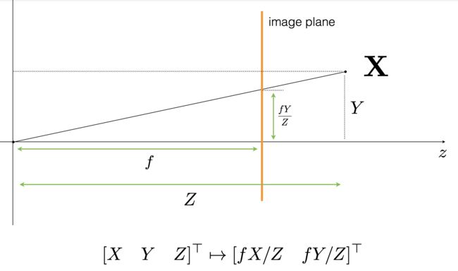
project_to_image calculates projected_pts_2d(nx3) = pts_3d_extended(nx4) dot P’(4x3). There are two mathematical process:

Ref this link for more detailed explanation of camera projection.

The project result is the 2D bounding box in the image coordinate: