Code of Deep Learning (Based on pytorch)
0. 机器学习数据预处理基础
One-Hot编码
- 使用Pandas中的value_counts()函数,查看data中的特征User continent的取值类型, 并打印输出的内容;
- 使用pandas中的get_dummies()函数对data中的特征User continent进行One-Hot编码,参数prefix为User continent_;
- 将编码后的结果保存在encode_uc中,并输出变量的前5行内容
import pandas as pd
data = pd.read_csv('user_review.csv')
# 请在下方作答 #
user_continent_counts = data['User continent'].value_counts()
print(user_continent_counts)
encoded_uc = pd.get_dummies(data['User continent'], prefix='User continent_')
print(encoded_uc.head())
缺失值填补
- 使用pandas中的value_counts()函数打印输出data中的特征Traveler type的取值统计信息, 并查看其是否含有缺失值;
- 如果存在缺失值,将特征Traveler type在其他样本中取值频数最多的值保存在变量freq_v中,并使用freq_v进行缺失值填充;
- 再次打印输出特征Traveler type的取值统计信息
# dropna=True:是否删除缺失值na默认删除
print(data['Traveler type'].value_counts(dropna=False))

# idxmax()函数用于沿索引轴查找最大值的索引。
freq_v = data['Traveler type'].value_counts(dropna=False).idxmax()
### 缺失值填充
#
data['Traveler type'] = data['Traveler type'].fillna(freq_v)

### 打印
print('')
print(u'缺失值填充完之后:')
print( '')
print(data['Traveler type'].value_counts(dropna=False))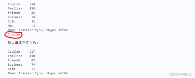
值得注意的是freq_v当中保存的是最大值,而不是其索引。然后在fillna()当中用该值对NaN进行填充。
特征标准化
- 使用sklearn中preprocessing模块下的StandardScaler()函数对data的特征Score进行Z-score标准化;
- 将特征取值的均值保存在变量score_mean中,并打印;
- 将特征取值的方差保存在变量score_var中,并打印。
std_scaler = StandardScaler() #注意需要将将其进行实例化

## Score特征标准化,使用fit_transform()方法
normal_df =std_scaler.fit_transform(data[['Score']])

## 均值
score_mean = normal_df.mean()

## 方差
score_var = normal_df.var()

## 打印
print (score_mean)
print (score_var)

## 打印前五行内容
normal_df[:5]- 自定义函数min_max()实现MinMax标准化,输入参数data为要进行标准化的数据,输出为标准化后的数据。
- 使自定义的min_max()函数对data的特征Score进行MinMax标准化,输出结果保存在score_transformed中,并打印变量的前5行内容
def min_max(data):

    ## 最小值
    data_min = data.min()
    ## 最大值
    data_max = data.max()
    ## 最大值与最小值之间的差值
    dv=data_max-data_min
    ## 根据MinMax标准化的定义实现
    new_data = (data-data_min)/dv

    ## 返回结果
    return new_data

## 调用min_max()函数
score_transformed = min_max(data['Score'])

## 打印变量的前5行内容
score_transformed.head()- 自定义logistic()函数,输入参数为要进行标准化的数据,输出结果为经过标准化后的数据;
- 使用自定义函数对data的特征Member years进行Logsitic标准化,结果保存在member_transformed中,并输出变量的前5行内容
def logistic(data):

    import numpy as np
    import warnings
    warnings.filterwarnings("ignore")

    ## 计算 1 + e^(-x)
    denominator =(1 + np.exp(-data))

    ## 实现logistic标准化
    new_data = 1/denominator
    ## 返回结果
    return new_data

## 对特征Member years进行logsitic标准化
member_transformed = logistic(data['Member years'])
## 打印内容
member_transformed.head()
特征离散化
- 使用Pandas的qcut()函数对data中的特征Member years进行等频离散化,结果保存在bins中;
- 使用pd.value_counts()函数统计categorical对象bins的取值信息。
离散化 (Discretization) (有些时候叫 量化(quantization) 或 装箱(binning)) 提供了将连续特征划分为离散特征值的方法。 某些具有连续特征的数据集会受益于离散化,因为 离散化可以把具有连续属性的数据集变换成只有名义属性(nominal attributes)的数据集。
chatgpt给出的例子

feature_to_discretize = 'Member years'
num_bins = 4

## 返回bins
bins,_ = pd.qcut(data[feature_to_discretize], q=num_bins, labels=None, retbins=True, duplicates='drop')

## 统计取值信息
print(bins.value_counts())
离群值检测
- 使用拉依达准则对data的特征Member years进行离群值检测;
- 如果存在离群值,输出离群值的个数outlier_num,并将包含离群值的数据记录保存在变量outeliers中,并打印变量内容。
import pandas as pd
import numpy as np
data = pd.read_csv('user_review.csv')
member_data = data[['Member years']]

# 请在下方作答 #
## Z-score标准化
std_scaler = StandardScaler()
new_data = std_scaler.fit_transform(member_data)


feature_to_detect_outliers = 'Member years'

# 计算四分位数
Q1 = data[feature_to_detect_outliers].quantile(0.25)
Q3 = data[feature_to_detect_outliers].quantile(0.75)
IQR = Q3 - Q1
inner_fence = 1.5 * IQR  # 内限
outer_fence = 3.0 * IQR  # 外限

## 写出过滤条件
outlier_judge = data[(data[feature_to_detect_outliers] < (Q1 - outer_fence)) | (data[feature_to_detect_outliers] > (Q3 + outer_fence))]

## 统计离群值的个数
outlier_num = len(outlier_judge)

## 包含离群值的数据样本记录
outliers = outlier_judge

## 打印
print(outliers)
1. 简单实现一个深度学习网络
参考:PyTorch深度学习快速入门教程(绝对通俗易懂!)【小土堆】_哔哩哔哩_bilibili
from  torch import  nn
from  torch.nn import Conv2d,MaxPool2d,Flatten,Linear,Sequential


import torchvision
from torch.utils.data import DataLoader


# 准备测试数据集
test_data = torchvision.datasets.CIFAR10("./dataCIT",train=False,transform=torchvision.transforms.ToTensor())


test_loader = DataLoader(dataset=test_data,batch_size=64,shuffle=True,num_workers=0,drop_last=False)

class Tudui(nn.Module):
    def __init__(self):
        super(Tudui,self).__init__()
        # self.conv1 =Conv2d(3,32,5,padding=2)
        # self.maxpool1=MaxPool2d(2)
        # self.conv2 = Conv2d(32, 32, 5, padding=2)
        # self.maxpool2 = MaxPool2d(2)
        # self.conv3 = Conv2d(32, 64, 5, padding=2)
        # self.maxpool3 = MaxPool2d(2)
        # self.flatten = Flatten()
        # self.linear1 =Linear(1024,64)
        # self.linear2 = Linear(64,10)

        # 利用Sequential改写
        self.model1 =Sequential(Conv2d(3,32,5,padding=2),
                                MaxPool2d(2),
                                Conv2d(32, 32, 5, padding=2),
                                MaxPool2d(2),
                                Conv2d(32, 64, 5, padding=2),
                                MaxPool2d(2),
                                Flatten(),
                                Linear(1024, 64),
                                Linear(64, 10),
                                )

    def forward(self,x):
        # x = self.conv1(x)
        # x = self.maxpool1(x)
        # x = self.conv2(x)
        # x = self.maxpool2(x)
        # x = self.conv3(x)
        # x = self.maxpool3(x)
        # x = self.flatten(x)
        # x = self.linear1(x)
        # x = self.linear2(x)

        x =self.model1(x)
        return x

# 定义loss
loss =nn.CrossEntropyLoss()

#搭建网络
tudui =Tudui()

# 选择随机梯度下降作为优化器

optim = torch.optim.SGD(tudui.parameters(),lr=0.01)

for epoch in range(20):
    running_loss=0.0
    for data in test_loader:
        img, targets = data
        outputs = tudui(img)
        result_loss = loss(outputs, targets)  # 计算loss
        optim.zero_grad()  # 对之前的梯度参数进行清零
        result_loss.backward()  # 反向传播
        optim.step()  # 使用优化器对于参数进行调优
        running_loss = running_loss+result_loss
    print(running_loss) # 相当于计算每轮的总loss
输出:
较为完整的训练过程
参考:PyTorch深度学习快速入门教程(绝对通俗易懂!)【小土堆】_哔哩哔哩_bilibili
import  torchvision
from torch.utils.data import  DataLoader
import torch
from torch import nn
from torch.nn import Conv2d,MaxPool2d,Flatten,Linear,Sequential


import torchvision
from torch.utils.data import DataLoader

class Tudui(nn.Module):
    def __init__(self):
        super(Tudui,self).__init__()
        # 不使用Sequential
        # self.conv1 =Conv2d(3,32,5,padding=2)
        # self.maxpool1=MaxPool2d(2)
        # self.conv2 = Conv2d(32, 32, 5, padding=2)
        # self.maxpool2 = MaxPool2d(2)
        # self.conv3 = Conv2d(32, 64, 5, padding=2)
        # self.maxpool3 = MaxPool2d(2)
        # self.flatten = Flatten()
        # self.linear1 =Linear(1024,64)
        # self.linear2 = Linear(64,10)

        # 利用Sequential改写
        self.model1 =Sequential(Conv2d(3,32,5,padding=2),
                                MaxPool2d(2),
                                Conv2d(32, 32, 5, padding=2),
                                MaxPool2d(2),
                                Conv2d(32, 64, 5, padding=2),
                                MaxPool2d(2),
                                Flatten(),
                                Linear(1024, 64),
                                Linear(64, 10),
                                )

    def forward(self,x):
        # x = self.conv1(x)
        # x = self.maxpool1(x)
        # x = self.conv2(x)
        # x = self.maxpool2(x)
        # x = self.conv3(x)
        # x = self.maxpool3(x)
        # x = self.flatten(x)
        # x = self.linear1(x)
        # x = self.linear2(x)

        x = self.model1(x)
        return x

if __name__ == '__main__':
    tudui =Tudui()
    input =torch.ones((64,3,32,32))
    output =tudui(input)
    print(output.shape)
import torchvision
from torch.utils.data import DataLoader
import torch
from torch import nn
from torch.nn import Conv2d,MaxPool2d,Flatten,Linear,Sequential
import torchvision
from torch.utils.data import DataLoader
from TuduiModel import *
# 准备数据集
train_data = torchvision.datasets.CIFAR10("./dataCIT",train=True,transform=torchvision.transforms.ToTensor())
test_data = torchvision.datasets.CIFAR10("./dataCIT",train=False,transform=torchvision.transforms.ToTensor())
# len长度
train_data_size = len(train_data)
test_data_size = len(test_data)
# 利用Dataloader来加载数据集
train_dataloader = DataLoader(dataset=train_data,batch_size=64,shuffle=True,num_workers=0,drop_last=False)
test_dataloader = DataLoader(dataset=test_data,batch_size=64,shuffle=True,num_workers=0,drop_last=False)
# 搭建神经网络
tudui = Tudui()
# 定义损失函数 这里由于是分类问题,所以使用了交叉熵作为损失函数
loss_fn =nn.CrossEntropyLoss()
# 定义优化器
learning_rate = 1e-2
optimizer = torch.optim.SGD(tudui.parameters(),lr=learning_rate)
#设置训练网络当中的一些参数
total_train_step =0 # 记录训练从次数
total_test_step =0 #记录测试的次数
epoch = 10 #训练的轮数
for i in range (epoch):
print("-------------第{}轮训练开始-------------".format(i+1))
for data in train_dataloader:
imgs,targets =data
outputs = tudui(imgs)
loss = loss_fn(outputs,targets)
#优化器优化模型
optimizer.zero_grad()
loss.backward()
optimizer.step()
total_train_step =total_train_step+1
if total_train_step% 100 ==0:
print("训练次数:{},Loss{}".format(total_train_step,loss.item()))
# 测试步骤
total_test_loss = 0
with torch.no_grad(): # 相当于不再对于梯度进行调优
for data in test_dataloader:
imgs,targets = data
output = tudui(imgs)
loss = loss_fn(output,targets)
total_test_loss =total_test_loss+loss
print("整体测试集上的loss:{}".format(total_test_loss))
增加accuracy后
import  torchvision
from torch.utils.data import  DataLoader
import torch
from  torch import  nn
from  torch.nn import Conv2d,MaxPool2d,Flatten,Linear,Sequential


import torchvision
from torch.utils.data import DataLoader
from TuduiModel import *

# 准备数据集
train_data = torchvision.datasets.CIFAR10("./dataCIT",train=True,transform=torchvision.transforms.ToTensor())
test_data = torchvision.datasets.CIFAR10("./dataCIT",train=False,transform=torchvision.transforms.ToTensor())

# len长度
train_data_size = len(train_data)
test_data_size = len(test_data)

# 利用Dataloader来加载数据集
train_dataloader = DataLoader(dataset=train_data,batch_size=64,shuffle=True,num_workers=0,drop_last=False)
test_dataloader = DataLoader(dataset=test_data,batch_size=64,shuffle=True,num_workers=0,drop_last=False)


# 搭建神经网络
tudui = Tudui()

# 定义损失函数 这里由于是分类问题,所以使用了交叉熵作为损失函数
loss_fn =nn.CrossEntropyLoss()

# 定义优化器
learning_rate = 1e-2
optimizer = torch.optim.SGD(tudui.parameters(),lr=learning_rate)

#设置训练网络当中的一些参数

total_train_step =0 # 记录训练从次数
total_test_step =0 #记录测试的次数
epoch = 10 #训练的轮数

# 开始训练

for i in range (epoch):
    print("-------------第{}轮训练开始-------------".format(i+1))
    tudui.train() #让网络进入训练状态
    for data in train_dataloader:
        imgs,targets =data
        outputs = tudui(imgs)
        loss = loss_fn(outputs,targets)
        #优化器优化模型
        optimizer.zero_grad()
        loss.backward()
        optimizer.step()
        total_train_step =total_train_step+1
        if total_train_step% 100 ==0:
            print("训练次数:{},Loss{}".format(total_train_step,loss.item()))

    # 测试步骤
    tudui.eval() #让网络进入测试状态
    total_test_loss = 0
    total_accuracy =0
    with torch.no_grad(): # 相当于不再对于梯度进行调优
        for data in test_dataloader:
            imgs,targets = data
            output = tudui(imgs)
            loss = loss_fn(output,targets)
            total_test_loss =total_test_loss+loss
            accuracy = (output.argmax(1)== targets).sum()
            total_accuracy =total_accuracy+accuracy
    print("整体测试集上的loss:{}".format(total_test_loss))
    print("整体测试集上的正确率:{}".format(total_accuracy/test_data_size))
使用GPU进行训练版本:
import  torchvision
from torch.utils.data import  DataLoader
import torch
from  torch import  nn
from  torch.nn import Conv2d,MaxPool2d,Flatten,Linear,Sequential


import torchvision
from torch.utils.data import DataLoader
from TuduiModel import *

# 准备数据集
train_data = torchvision.datasets.CIFAR10("./dataCIT",train=True,transform=torchvision.transforms.ToTensor())
test_data = torchvision.datasets.CIFAR10("./dataCIT",train=False,transform=torchvision.transforms.ToTensor())

# len长度
train_data_size = len(train_data)
test_data_size = len(test_data)

# 利用Dataloader来加载数据集
train_dataloader = DataLoader(dataset=train_data,batch_size=64,shuffle=True,num_workers=0,drop_last=False)
test_dataloader = DataLoader(dataset=test_data,batch_size=64,shuffle=True,num_workers=0,drop_last=False)


# 搭建神经网络
tudui = Tudui()
# if torch.cuda.is_available(): 如果未知是否有GPU,可以先进行判断
tudui=tudui.cuda()  # 将模型的训练转移到GPU上

# 定义损失函数 这里由于是分类问题,所以使用了交叉熵作为损失函数
loss_fn =nn.CrossEntropyLoss()
loss_fn = loss_fn.cuda() #将Loss的计算放到GPU当中

# 定义优化器
learning_rate = 1e-2
optimizer = torch.optim.SGD(tudui.parameters(),lr=learning_rate)


#设置训练网络当中的一些参数

total_train_step =0 # 记录训练从次数
total_test_step =0 #记录测试的次数
epoch = 10 #训练的轮数

# 开始训练

for i in range (epoch):
    print("-------------第{}轮训练开始-------------".format(i+1))
    tudui.train() #让网络进入训练状态
    for data in train_dataloader:
        imgs,targets =data
        imgs = imgs.cuda()
        targets = targets.cuda()
        outputs = tudui(imgs)
        loss = loss_fn(outputs,targets)
        #优化器优化模型
        optimizer.zero_grad()
        loss.backward()
        optimizer.step()
        total_train_step =total_train_step+1
        if total_train_step% 100 ==0:
            print("训练次数:{},Loss{}".format(total_train_step,loss.item()))

    # 测试步骤
    tudui.eval() #让网络进入测试状态
    total_test_loss = 0
    total_accuracy =0
    with torch.no_grad(): # 相当于不再对于梯度进行调优
        for data in test_dataloader:
            imgs,targets = data
            imgs =imgs.cuda()
            targets =targets.cuda()
            output = tudui(imgs)
            loss = loss_fn(output,targets)
            total_test_loss =total_test_loss+loss
            accuracy = (output.argmax(1)== targets).sum()
            total_accuracy =total_accuracy+accuracy
    print("整体测试集上的loss:{}".format(total_test_loss))
    print("整体测试集上的正确率:{}".format(total_accuracy/test_data_size))
2. 使用CIFAR10实现图像识别
CIFAR-10 数据集包括 60000 张 32x32 的彩色图像,分为 10 个类别,每个类别包含 6000 张图像。其中,50000 张图像用于训练,10000 张图像用于测试。
模型训练
import torchvision
from torch.utils.data import DataLoader
import torch
from torch import nn
from torch.nn import Conv2d,MaxPool2d,Flatten,Linear,Sequential
import torchvision
from torch.utils.data import DataLoader
from TuduiModel import *
# 准备数据集
train_data = torchvision.datasets.CIFAR10("./dataCIT",train=True,transform=torchvision.transforms.ToTensor())
test_data = torchvision.datasets.CIFAR10("./dataCIT",train=False,transform=torchvision.transforms.ToTensor())
# len长度
train_data_size = len(train_data)
test_data_size = len(test_data)
# 利用Dataloader来加载数据集
train_dataloader = DataLoader(dataset=train_data,batch_size=64,shuffle=True,num_workers=0,drop_last=False)
test_dataloader = DataLoader(dataset=test_data,batch_size=64,shuffle=True,num_workers=0,drop_last=False)
# 搭建神经网络
tudui = Tudui()
# if torch.cuda.is_available(): 如果未知是否有GPU,可以先进行判断
tudui=tudui.cuda() # 将模型的训练转移到GPU上
# 定义损失函数 这里由于是分类问题,所以使用了交叉熵作为损失函数
loss_fn =nn.CrossEntropyLoss()
loss_fn = loss_fn.cuda() #将Loss的计算放到GPU当中
# 定义优化器
learning_rate = 1e-2
optimizer = torch.optim.SGD(tudui.parameters(),lr=learning_rate)
#设置训练网络当中的一些参数
total_train_step =0 # 记录训练从次数
total_test_step =0 #记录测试的次数
epoch = 60 #训练的轮数
# 开始训练
for i in range (epoch):
print("-------------第{}轮训练开始-------------".format(i+1))
tudui.train() #让网络进入训练状态
for data in train_dataloader:
imgs,targets =data
imgs = imgs.cuda()
targets = targets.cuda()
outputs = tudui(imgs)
loss = loss_fn(outputs,targets)
#优化器优化模型
optimizer.zero_grad()
loss.backward()
optimizer.step()
total_train_step =total_train_step+1
if total_train_step% 100 ==0:
print("训练次数:{},Loss{}".format(total_train_step,loss.item()))
# 测试步骤
tudui.eval() #让网络进入测试状态
total_test_loss = 0
total_accuracy =0
with torch.no_grad(): # 相当于不再对于梯度进行调优
for data in test_dataloader:
imgs,targets = data
imgs =imgs.cuda()
targets =targets.cuda()
output = tudui(imgs)
loss = loss_fn(output,targets)
total_test_loss =total_test_loss+loss
accuracy = (output.argmax(1)== targets).sum()
total_accuracy =total_accuracy+accuracy
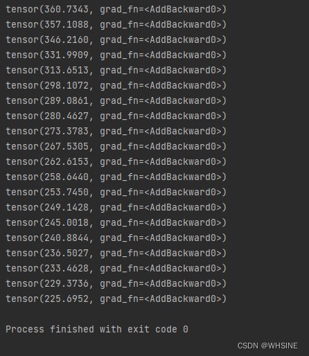
print("整体测试集上的loss:{}".format(total_test_loss))
print("整体测试集上的正确率:{}".format(total_accuracy/test_data_size))
torch.save(tudui,"tudui_{}.pth".format(60))
print("模型已保存")模型预测
import  torchvision
from torch.utils.data import  DataLoader
import torch
from torch import nn
from torch.nn import Conv2d,MaxPool2d,Flatten,Linear,Sequential
from  PIL import  Image


import torchvision
from torch.utils.data import DataLoader
image_path = "testPic/img_5.png"
image = Image.open(image_path)
image = image.convert('RGB')
transform = torchvision.transforms.Compose([torchvision.transforms.Resize((32, 32)),
                                            torchvision.transforms.ToTensor()])
image = transform(image)
image = image.cuda()

#
# class Tudui(nn.Module):
#     def __init__(self):
#         super(Tudui, self).__init__()
#         self.model = nn.Sequential(
#             nn.Conv2d(3, 32, 5, 1, 2),
#             nn.MaxPool2d(2),
#             nn.Conv2d(32, 32, 5, 1, 2),
#             nn.MaxPool2d(2),
#             nn.Conv2d(32, 64, 5, 1, 2),
#             nn.MaxPool2d(2),
#             nn.Flatten(),
#             nn.Linear(64*4*4, 64),
#             nn.Linear(64, 10)
#         )
#
#     def forward(self, x):
#         x = self.model(x)
#         return x

model =torch.load("tudui_60.pth",)
image =torch.reshape(image,(1,3,32,32))
model.eval()
with torch.no_grad():
    output = model(image)
    Max_Value = torch.max(output)
    max_index = torch.argmax(output)
    max_index_item = max_index.item()
# if max_index_item == 0:
#     print("此图片当中的物体是飞机")
# elif max_index_item ==1:
#     print("此图片当中的物体是汽车")
# elif max_index_item ==2:
#     print("此图片当中的物体是鸟")
# elif max_index_item ==3:
#     print("此图片当中的物体是猫")
# elif max_index_item ==4:
#     print("此图片当中的物体是鹿")
# elif max_index_item ==5:
#     print("此图片当中的物体是狗")
# elif max_index_item ==6:
#     print("此图片当中的物体是青蛙")
# elif max_index_item ==7:
#     print("此图片当中的物体是马")
# elif max_index_item ==8:
#     print("此图片当中的物体是船")
# elif max_index_item ==9:
#     print("此图片当中的物体卡车")

# 创建一个字典,将索引值映射到对应的物体名称
class_map = {
    0: "飞机",
    1: "汽车",
    2: "鸟",
    3: "猫",
    4: "鹿",
    5: "狗",
    6: "青蛙",
    7: "马",
    8: "船",
    9: "卡车"
}

# 使用字典查找索引对应的物体名称
if max_index_item in class_map:
    object_name = class_map[max_index_item]
    print(f"此图片当中的物体是{object_name}")
else:
    print("未知物体")
训练效果:
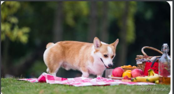
以该图片为例,当设置模型训练epoch为40时,无法成功识别 :(
当设置模型训练epoch为60时,成功识别柯基:)
预测模型改进空间:
可以使用更大的训练数据集;
可以使用效果更好的训练模型;
现有只可以对CIFAR-10当中标注的10个类别进行预测,难以对更多的物体类别进行预测。
3. Pytorch当中Dataset和Dataloader类的使用
# 首先想要构建自己的Dataset类 需要继承pytorch官方的Dataset类,同时自定义的Dataset类必须实现__init__, _len_, 和__getitem__
#A custom Dataset class must implement three functions: __init__, __len__, and __getitem__.

# Dataset
# Pytorch 官方Dataset示例代码
import os
import pandas as pd
from torch.utils.data import Dataset
from torch.utils.data import DataLoader
from torchvision.io import read_image

class CustomImageDataset(Dataset):
    # The __init__ function is run once when instantiating the Dataset object.
    def __init__(self, annotations_file, img_dir, transform=None, target_transform=None):
        self.img_labels = pd.read_csv(annotations_file) # annotations_file 这个文件当中相当于存储着图片的名称信息和其对应的label信息
        self.img_dir = img_dir # 存储图片的文件夹
        self.transform = transform # 可以自定义一个对于图像进行预处理的函数
        self.target_transform = target_transform # 可以自定义一个对于标签进行预处理的函数

    # The __len__ function returns the number of samples in our dataset.

    def __len__(self):
        return len(self.img_labels)

    # The __getitem__ function loads and returns a sample from the dataset at the given index idx
    def __getitem__(self, idx):
        # 对图片的地址进行拼接
        img_path = os.path.join(self.img_dir, self.img_labels.iloc[idx, 0]) # Pandas DataFrame对象上的一种索引和访问方式,用于从DataFrame中获取特定位置的数据。是Pandas DataFrame对象上的索引器,它用于通过行和列的整数位置来访问数据
        image = read_image(img_path)
        label = self.img_labels.iloc[idx, 1]
        if self.transform:
            image = self.transform(image)
        if self.target_transform:
            label = self.target_transform(label)
        return image, label

training_data = CustomImageDataset()
test_data =CustomImageDataset()


# Dataloader
# reparing your data for training with DataLoaders
# The Dataset retrieves our dataset’s features and labels one sample at a time. While training a model, we typically want to pass samples in “minibatches”, reshuffle the data at every epoch to reduce model overfitting, and use Python’s multiprocessing to speed up data retriev
# 数据集(Dataset)一次获取我们数据集的一个样本的特征和标签。
# 在训练模型时,通常希望以“小批量”(minibatches)的方式传递样本,每个时期重新洗牌数据以减少模型过拟合,并使用Python的多进程(multiprocessing)加速数据获取。

# 示例代码
train_dataloader = DataLoader(training_data, batch_size=64, shuffle=True)
test_dataloader = DataLoader(test_data, batch_size=64, shuffle=True)
import torch
from torchvision import datasets
from torchvision.transforms import ToTensor, Lambda
from torchvision import transforms
from PIL import Image
# Data does not always come in its final processed form that is required for training machine learning algorithms.
# We use transforms to perform some manipulation of the data and make it suitable for training.
# All TorchVision datasets have two parameters -transform to modify the features
# and target_transform to modify the label
# transform类似一个工具箱
# 使用transform需要关注输入和输出,需要关注方法需要什么参数
# transform.Totensor Totensor的使用是将一个PIL Image或者numpy.ndarray转变为tensor
img_path = "hymenoptera_data/train/ants/0013035.jpg"
img =Image.open(img_path)
# 将图片转化为张量
tensor_trans = transforms.ToTensor()# 相当于利用transform这个工具箱创建了一个自己的工具
tensor_img =tensor_trans(img)
#print(tensor_img)
# Normalize Normalize a tensor image with mean and stand deviation
trans_norm = transforms.Normalize([0.5,0.5,0.5],[0.5,0.5,0.5]) # 是PyTorch中的一个图像转换函数,它用于对图像的每个通道进行标准化(normalize)。这个函数通常用于在深度学习模型的训练中对输入数据进行预处理,以便提高模型的训练效果
img_norm =trans_norm(tensor_img)
# Resize Resize the input PIL Image to the given size
print(img.size)
trans_resize = transforms.Resize((512,512))
img_resize =trans_resize(img)
img_resize =tensor_trans(img_resize)
print(img_resize)
# Compose
#使用transforms.Compose创建了一个组合的图像变换。transforms.Compose 允许你将多个图像变换按顺序组合在一起,以便在一次操作中应用它们。在这个例子中,首先应用了trans_resize_2来将图像调整为512x512像素的大小,然后应用了tensor_trans来将其转换为PyTorch张量。
trans_resize_2 = transforms.Resize(512)
trans_compose = transforms.Compose([trans_resize_2,tensor_trans])
img_resize_2 = trans_compose(img)
# pytorch官方示例
ds = datasets.FashionMNIST(
root="data",
train=True,
download=True,
transform=ToTensor(),
target_transform=Lambda(lambda y: torch.zeros(10, dtype=torch.float).scatter_(0, torch.tensor(y), value=1))
)
# target_transform=Lambda(lambda y: torch.zeros(10, dtype=torch.float).scatter_(0, torch.tensor(y), value=1))含义:
# 这段代码似乎是为了将标签数据从一个类别索引的形式转换为独热编码(one-hot encoding)的形式。一般情况下,神经网络在训练过程中常用独热编码来表示类别标签,其中每个类别都被编码为一个二进制向量,只有对应类别的位置为1,其他位置为0。
# 这里使用了PyTorch的张量操作来执行这个转换。让我们分解代码的不同部分:
# target_transform=:这是一个参数,通常用于数据集对象,以指定如何转换标签数据。
# Lambda(lambda y: ...):这部分使用Python的lambda函数创建一个匿名函数,该函数接受一个参数y,即原始的类别标签。
# torch.zeros(10, dtype=torch.float):这个部分创建了一个包含10个零的张量,数据类型为浮点型。
#.scatter_(0, torch.tensor(y), value=1):这是一个张量操作,它将1的值散布到张量的特定位置。具体地说,它将标签y处的位置设置为1,而其他位置保持为0。0参数表示维度0,torch.tensor(y)表示要在哪个位置设置1,value=1表示要设置的值为1。
# 综合起来,这段代码的目的是将原始的类别标签 y 转换为一个长度为10的独热编码张量,其中对应类别的位置为1,其他位置为0。这个转换通常用于多类别分类问题,其中有10个类别,每个类别由一个索引标识,而模型需要以独热编码的形式来处理这些标签。4. Pytorch当中的transforms的使用
import torch
from torchvision import datasets
from torchvision.transforms import ToTensor, Lambda
from  torchvision import transforms
from PIL import Image


# Data does not always come in its final processed form that is required for training machine learning algorithms.
# We use transforms to perform some manipulation of the data and make it suitable for training.
# All TorchVision datasets have two parameters -transform to modify the features
# and target_transform to modify the label

# transform类似一个工具箱
# 使用transform需要关注输入和输出,需要关注方法需要什么参数

# transform.Totensor Totensor的使用是将一个PIL Image或者numpy.ndarray转变为tensor

img_path = "hymenoptera_data/train/ants/0013035.jpg"
img =Image.open(img_path)

# 将图片转化为张量
tensor_trans = transforms.ToTensor()# 相当于利用transform这个工具箱创建了一个自己的工具
tensor_img =tensor_trans(img)
#print(tensor_img)


# Normalize  Normalize a tensor image with mean and stand deviation
trans_norm = transforms.Normalize([0.5,0.5,0.5],[0.5,0.5,0.5]) #  是PyTorch中的一个图像转换函数,它用于对图像的每个通道进行标准化(normalize)。这个函数通常用于在深度学习模型的训练中对输入数据进行预处理,以便提高模型的训练效果
img_norm =trans_norm(tensor_img)


# Resize Resize the input PIL Image to the given size

print(img.size)
trans_resize = transforms.Resize((512,512))
img_resize =trans_resize(img)
img_resize =tensor_trans(img_resize)
print(img_resize)

# Compose
#使用transforms.Compose创建了一个组合的图像变换。transforms.Compose 允许你将多个图像变换按顺序组合在一起,以便在一次操作中应用它们。在这个例子中,首先应用了trans_resize_2来将图像调整为512x512像素的大小,然后应用了tensor_trans来将其转换为PyTorch张量。
trans_resize_2 = transforms.Resize(512)
trans_compose = transforms.Compose([trans_resize_2,tensor_trans])
img_resize_2 = trans_compose(img)

# pytorch官方示例
ds = datasets.FashionMNIST(
    root="data",
    train=True,
    download=True,
    transform=ToTensor(),
    target_transform=Lambda(lambda y: torch.zeros(10, dtype=torch.float).scatter_(0, torch.tensor(y), value=1))
)

# target_transform=Lambda(lambda y: torch.zeros(10, dtype=torch.float).scatter_(0, torch.tensor(y), value=1))含义:
# 这段代码似乎是为了将标签数据从一个类别索引的形式转换为独热编码(one-hot encoding)的形式。一般情况下,神经网络在训练过程中常用独热编码来表示类别标签,其中每个类别都被编码为一个二进制向量,只有对应类别的位置为1,其他位置为0。

# 这里使用了PyTorch的张量操作来执行这个转换。让我们分解代码的不同部分:

# target_transform=:这是一个参数,通常用于数据集对象,以指定如何转换标签数据。

# Lambda(lambda y: ...):这部分使用Python的lambda函数创建一个匿名函数,该函数接受一个参数y,即原始的类别标签。

# torch.zeros(10, dtype=torch.float):这个部分创建了一个包含10个零的张量,数据类型为浮点型。

#.scatter_(0, torch.tensor(y), value=1):这是一个张量操作,它将1的值散布到张量的特定位置。具体地说,它将标签y处的位置设置为1,而其他位置保持为0。0参数表示维度0,torch.tensor(y)表示要在哪个位置设置1,value=1表示要设置的值为1。

# 综合起来,这段代码的目的是将原始的类别标签 y 转换为一个长度为10的独热编码张量,其中对应类别的位置为1,其他位置为0。这个转换通常用于多类别分类问题,其中有10个类别,每个类别由一个索引标识,而模型需要以独热编码的形式来处理这些标签。5. Pytorch 当中的nn.Module 类
# Neural networks comprise of layers/modules that perform operations on data.
# The torch.nn namespace provides all the building blocks you need to build your own neural network.
# Every module in PyTorch subclasses the nn.Module.
# A neural network is a module itself that consists of other modules (layers).
# #This nested structure allows for building and managing complex architectures easily

# 神经网络由对数据执行操作的层/模块组成。
# torch.nn 命名空间提供了构建自己的神经网络所需的所有基本组件。
# PyTorch 中的每个模块都是 nn.Module 的子类。
# 神经网络本身也是一个模块,它由其他模块(层)组成。
# 这种嵌套结构使得轻松构建和管理复杂的体系结构成为可能

import os
import torch
from torch import nn
from torch.utils.data import DataLoader
from torchvision import datasets, transforms

# Get Device for training
# We want to be able to train our model on a hardware accelerator like the GPU or MPS, if available.
# Let’s check to see if torch.cuda or torch.backends.mps are available, otherwise we use the CPU.

device = (
    "cuda"
    if torch.cuda.is_available()
    else "mps"
    if torch.backends.mps.is_available()
    else "cpu"
)

# 定义了一个类
# 值得注意的是,这个类继承于nn.Module
class NeuralNetwork(nn.Module):
    def __init__(self):
        super().__init__() # 表示调用了父类的方法
        self.flatten = nn.Flatten()

        # nn.Sequential相当于可以将括号当中的层进行自动的串联
        self.linear_relu_stack = nn.Sequential(
            nn.Linear(28*28, 512), # 第一个参数表示输入层的特征维度,第二个参数表示隐藏层的大小
            nn.ReLU(),   # 非线性层激活函数
            nn.Linear(512, 512),
            nn.ReLU(),
            nn.Linear(512, 10),
        )

    # forward 函数不需要去进行显示的调用

    def forward(self, x):
        x = self.flatten(x)
        logits = self.linear_relu_stack(x)
        return logits
# To use the model, we pass it the input data.
# This executes the model’s forward, along with some background operations. Do not call model.forward() directly!

# We create an instance of NeuralNetwork, and move it to the device, and print its structure.
model = NeuralNetwork().to(device)
print(model)

X = torch.rand(1, 28, 28, device=device)
logits = model(X)
pred_probab = nn.Softmax(dim=1)(logits) # 对 logits 进行 softmax 操作,将其转换为概率分布。Softmax 操作使得每个类别的输出变为0到1之间的概率,使得它们的总和等于1。
y_pred = pred_probab.argmax(1) # 这一行代码找到具有最高概率的类别索引,即对每个样本找到最有可能的类别
print(f"Predicted class: {y_pred}")

# nn.Flatten的用法
input_image = torch.rand(3,28,28)
flatten = nn.Flatten()
flat_image = flatten(input_image)
print(flat_image.size())
nn.Flatten的用法

第一个参数是开始flatten的维度,第二个参数是结束flatten的维度
import torch
from torch import nn
input_image = torch.rand(8,8,28,28)
flatten = nn.Flatten(1,2)
flat_image = flatten(input_image)
print(flat_image.size())![]()
import torch
from torch import nn
input_image = torch.rand(8,8,28,28)
flatten = nn.Flatten()
flat_image = flatten(input_image)
print(flat_image.size())![]()
nn.linear的用法
import torch
from torch import nn
# The linear layer is a module that applies a linear transformation on the input using its stored weights and biases.
# 第一个参数表示线性层接受的输入特征的维度,
# 第二个参数表示输出特征特征的维度
m = nn.Linear(20, 30)
input = torch.randn(99, 20)# 表示有99个样本,每个样本包含20维的特征
output = m(input)
print(output.size())![]() 值得注意的是: 输入的input的特征维度需要等于线性层一个参数
值得注意的是: 输入的input的特征维度需要等于线性层一个参数
nn.RELU的用法
print(f"Before ReLU: {hidden1}\n\n")
hidden1 = nn.ReLU()(hidden1) # 注意。在使用是需要对RELU()类进行实例化
print(f"After ReLU: {hidden1}")
nn.Sequential的用法
import torch
from torch import nn
# nn.Sequential is an ordered container of modules. The data is passed through all the modules in the same order as defined.
# You can use sequential containers to put together a quick network like seq_modules.
seq_modules = nn.Sequential(
    flatten,
    layer1,
    nn.ReLU(),
    nn.Linear(20, 10)
)
input_image = torch.rand(3,28,28)
logits = seq_modules(input_image)
nn.Sequential相当于是一个容器
6. 深度学习当中的线性回归
import torch
import random


# 构建训练数据集
def Dataset(w,b,num_examples):
    X = torch.normal(0,1,(num_examples,len(w))) # 随机生成满足正态分布的数据
    y = torch.matmul(X,w)+b
    y += torch.normal(0,0.01,y.shape)
    return X,y.reshape((-1,1))


true_w =torch.tensor([2,-3.4])
true_b = 4.2
features, labels = Dataset(true_w,true_b,1000)


# 定义dataloader
def data_iter(batch_size,features,labels):
     num_examples = len(features)
     indices = list(range(num_examples))
     random.shuffle(indices)
     for i in range(0,num_examples,batch_size):
         batch_index = torch.tensor(indices[i:min(i+batch_size,num_examples)])
         # yield 是用于定义生成器(generator)的关键字,用于创建一个特殊的迭代器。
         # 生成器是一种能够生成一系列值的函数,但与普通函数不同,它可以保存函数的状态并在需要时按需生成值,
         # 而不是一次性生成所有值并将它们存储在内存中。
         yield features[batch_index],labels[batch_index]

# 初始化模型参数
w = torch.normal(0,0.01,size=(2,1),requires_grad=True)
b = torch.zeros(1,requires_grad=True)


# 定义模型
def linreg(x,w,b):
    return torch.matmul(x,w)+b
#定义损失函数
def squared_loss(y_hat, y):  #@save
    """均方损失"""
    return (y_hat - y.reshape(y_hat.shape)) ** 2
#定义优化器
def sgd(params, lr, batch_size):  #@save
    """小批量随机梯度下降"""
    with torch.no_grad(): # 上下文管理器的作用是将其内部的操作标记为不需要梯度信息
        for param in params:
            param -= lr * param.grad / batch_size
            param.grad.zero_()

lr = 0.03
num_epochs = 3
net = linreg
loss = squared_loss
batch_size = 10

for epoch in range(num_epochs):
    for X, y in data_iter(batch_size, features, labels):
        l = loss(net(X, w, b), y)  # X和y的小批量损失
        # 因为l形状是(batch_size,1),而不是一个标量。l中的所有元素被加到一起,
        # 并以此计算关于[w,b]的梯度
        l.sum().backward()
        sgd([w, b], lr, batch_size)  # 使用参数的梯度更新参数
    with torch.no_grad():
        train_l = loss(net(features, w, b), labels)
        print(f'epoch {epoch + 1}, loss {float(train_l.mean()):f}')
7. 分类问题当中的分类精度
import torch
from IPython import display
from d2l import torch as d2l
import matplotlib.pyplot as plt

import os

y = torch.tensor([0, 2])
y_hat = torch.tensor([[0.1, 0.3, 0.6], [0.3, 0.2, 0.5]])
# y_hat_max = y_hat.argmax(axis=1)
# print(y_hat_max)
# print(y_hat_max.type)


# 分类精度
def accuracy(y_hat, y):  #@save
    """计算预测正确的数量"""
    # 如果y_hat是矩阵,那么假定第二个维度存储每个类的预测分数。
    # 我们使用argmax获得每行中最大元素的索引来获得预测类别。
    # 然后我们将预测类别与真实y元素进行比较。
    if len(y_hat.shape) > 1 and y_hat.shape[1] > 1:
        # .argmax() 是一个张量方法,用于找到张量中具有最大值的元素的索引
        y_hat = y_hat.argmax(axis=1)

        #由于等式运算符“ == ”对数据类型很敏感,
        # 因此我们将y_hat的数据类型转换为与y的数据类型一致。
        # 结果是一个包含0(错)和1(对)的张量
    cmp = y_hat.type(y.dtype) == y

    return float(cmp.type(y.dtype).sum())

print(accuracy(y_hat, y) / len(y))
8. SoftMax
# 定义softmax计算方法
def softmax(X):
    X_exp = torch.exp(X)
    partition = X_exp.sum(1, keepdim=True)
    return X_exp / partition  # 这里应用了广播机制

X = torch.normal(0, 1, (2, 5))
X_prob = softmax(X)
X_prob, X_prob.sum(1)
