机器学习2022吴恩达老师课程——学习笔记（二）

监督学习的最基本的类型——线性回归（Linear Regression）

线性回归的最简单的一种——Linear Regression with One Variable

关于Model Representation(代码）:

(Learn to implement the model    for linear regression with one variabl)

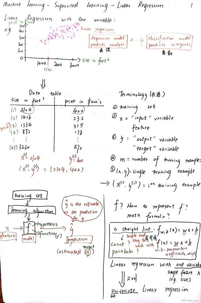
假设数据集中只有两个样本点：

Python代码——线性回归模型

 1.导入numpy和matplotlib

import numpy as np
import matplotlib.pyplot as plt
plt.style.use('./deeplearning.mplstyle')

2.create x_train and y_train variables（样本点的x值和y值）

# x_train is the input variable (size in 1000 square feet)
# y_train is the target (price in 1000s of dollars)
x_train = np.array([1.0, 2.0])
y_train = np.array([300.0, 500.0])
print(f"x_train = {x_train}")
print(f"y_train = {y_train}")

输出：

 3.获得样本点数量m(此例中m=2)

# m is the number of training examples
print(f"x_train.shape: {x_train.shape}")
m = x_train.shape[0]
print(f"Number of training examples is: {m}")

输出：

关于 x_train.shape 的理解：

举例：

（1）b=np.array([1,2,3])   print(b.shape)  输出：（3，）

（2）a=np.array([[1,2,5],[3,4,6]])  print(a.shape)  输出：（2，3）

（3）d = np.array([[[1,2,5],[3,4,6]]])  print(a.shape)  输出：(1, 2, 3)

或者

# m is the number of training examples
m = len(x_train)
print(f"Number of training examples is: {m}")

 4.样本点

for i in range(2):
    x_i = x_train[i]
    y_i = y_train[i]
    print(f"(x^({i}), y^({i})) = ({x_i}, {y_i})")

输出：

 5.绘制样本点

# Plot the data points
plt.scatter(x_train, y_train, marker='x', c='r')
# Set the title
plt.title("Housing Prices")
# Set the y-axis label
plt.ylabel('Price (in 1000s of dollars)')
# Set the x-axis label
plt.xlabel('Size (1000 sqft)')
plt.show()

• plt.scatter(x,y,marker,c)  画点，x,y是需要绘制的数据点，marker是标记的样式（'x'表示叉叉），c是绘制的color(r代表red)
• plt.title() 图表的标题
• plt.ylabel() y轴的坐标
• plt.xlabel() x轴的坐标
• plt.show() 显示

图： 

 6.绘制f(x)=wx+b  (Let's start with w=100 and b=100.)

构造函数compute_model_output来计算f_wb:

def compute_model_output(x, w, b):
    """
    Computes the prediction of a linear model
    Args:
      x (ndarray (m,)): Data, m examples 
      w,b (scalar)    : model parameters  
    Returns
      y (ndarray (m,)): target values
    """
    m = x.shape[0]
    f_wb = np.zeros(m)
    for i in range(m):
        f_wb[i] = w * x[i] + b
        
    return f_wb

w = 100
b = 100

tmp_f_wb = compute_model_output(x_train, w, b,)

# Plot our model prediction
plt.plot(x_train, tmp_f_wb, c='b',label='Our Prediction')

# Plot the data points
plt.scatter(x_train, y_train, marker='x', c='r',label='Actual Values')

# Set the title
plt.title("Housing Prices")
# Set the y-axis label
plt.ylabel('Price (in 1000s of dollars)')
# Set the x-axis label
plt.xlabel('Size (1000 sqft)')
plt.legend()
plt.show()

• plt.plot(x,y,c,label)  画线，x为x轴数据，y为y轴数据，c为线的color，label为线的标签
• plt.legend() 加上这个才能使标签显示出来

 图：

 7.根据模型做出预测

w = 200                         
b = 100    
x_i = 1.2
cost_1200sqft = w * x_i + b    

print(f"${cost_1200sqft:.0f} thousand dollars")

输出：

这部分还是比较简单比较好理解！ 

Python代码——成本函数

1.一些import啥的 

%matplotlib widge 交互式可视化图表，需要安装ipywidgets模块(这个安装还挺费时间的）

import numpy as np
%matplotlib widget
import matplotlib.pyplot as plt
from lab_utils_uni import plt_intuition, plt_stationary, plt_update_onclick, soup_bowl
plt.style.use('deeplearning.mplstyle')

2.训练数据（还是两个样本点）

x_train = np.array([1.0, 2.0])           #(size in 1000 square feet)
y_train = np.array([300.0, 500.0])           #(price in 1000s of dollars)

3.计算成本的函数（最小二乘法）

def compute_cost(x, y, w, b): 
    """
    Computes the cost function for linear regression.
    
    Args:
      x (ndarray (m,)): Data, m examples 
      y (ndarray (m,)): target values
      w,b (scalar)    : model parameters  
    
    Returns
        total_cost (float): The cost of using w,b as the parameters for linear regression
               to fit the data points in x and y
    """
    # number of training examples
    m = x.shape[0] 
    
    cost_sum = 0 
    for i in range(m): 
        f_wb = w * x[i] + b   
        cost = (f_wb - y[i]) ** 2  
        cost_sum = cost_sum + cost  
    total_cost = (1 / (2 * m)) * cost_sum  

    return total_cost

4.生成交互式可视化图表

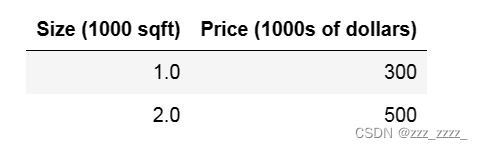
plt_intuition(x_train,y_train)

（一开始运行的时候，只有两个图表的矩形区域，并没有曲线、直线啥的，然后下面显示报错是： AttributeError: Unknown property ls，一开始也不知道怎么弄，查了 ax.vlines方法中也存在着ls属性，我试着把 ls='dotted'删掉了。再运行竟然出来了（如下图），就是紫色那个有dotted的是虚线而我删掉之后变成了实线）

这部分代码（有很多函数调用）比较复杂，但目的是生成两个图，一个是x与y的坐标图（包含样本点和线性回归模型），另一个是取得的W和对应的成本之间的关系，可以看出是一个碗状的抛物线。

注意：已设b=100。

 5.更复杂的数据样本

x_train = np.array([1.0, 1.7, 2.0, 2.5, 3.0, 3.2])
y_train = np.array([250, 300, 480,  430,   630, 730,])

 这里不再限制b是否等于一个固定的值

from mpl_toolkits.mplot3d import Axes3D
plt.close('all') 
fig, ax, dyn_items = plt_stationary(x_train, y_train)
updater = plt_update_onclick(fig, ax, x_train, y_train, dyn_items)

（运行的时候还是遇到AttributeError: Unknown property ls的报错，我把所有的ls='dotted'都删掉了，在此之前，还遇到了ValueError: Unknown projection ‘3d‘的错误，经过查阅，解决方法是在前面加上了from mpl_toolkits.mplot3d import Axes3D）

下面这三个图，上面第一个就是样本点和构造的线性回归模型（f(x)=w*x+b)以及可视化的error

上面第二个横轴是w，纵轴是b，其实应该是一个就像初中地理课本中的等高线图那样的（但我也不知道我这个怎么是这样）

下面那个就是取不同值对应的成本J（像一个吊床），其实和上面第二个是不同的表示而已，本质是一样的

soup_bowl()

 直观感知线性回归模型的w,b以及成本J