练习题目录
习题编号 内容 相应数据集
- 练习6 - 统计 探索风速数据 wind.data
- 练习7 - 可视化 探索泰坦尼克灾难数据 train.csv
- 练习8 - 创建数据框 探索Pokemon数据 练习中手动内置的数据
- 练习9 - 时间序列 探索Apple公司股价数据 Apple_stock.csv
- 练习10 - 删除数据 探索Iris纸鸢花数据 iris.csv
练习6-统计
探索风速数据
步骤1 导入必要的库
import pandas as pd
import datetime
步骤2 从以下地址导入数据
path6 = "./exercise_data/wind.data"
步骤3 将数据作存储并且设置前三列为合适的索引
import datetime
data = pd.read_table(path6, sep = "\s+", parse_dates = [[0,1,2]])
data.head()
|
Yr_Mo_Dy |
RPT |
VAL |
ROS |
KIL |
SHA |
BIR |
DUB |
CLA |
MUL |
CLO |
BEL |
MAL |
| 0 |
2061-01-01 |
15.04 |
14.96 |
13.17 |
9.29 |
NaN |
9.87 |
13.67 |
10.25 |
10.83 |
12.58 |
18.50 |
15.04 |
| 1 |
2061-01-02 |
14.71 |
NaN |
10.83 |
6.50 |
12.62 |
7.67 |
11.50 |
10.04 |
9.79 |
9.67 |
17.54 |
13.83 |
| 2 |
2061-01-03 |
18.50 |
16.88 |
12.33 |
10.13 |
11.17 |
6.17 |
11.25 |
NaN |
8.50 |
7.67 |
12.75 |
12.71 |
| 3 |
2061-01-04 |
10.58 |
6.63 |
11.75 |
4.58 |
4.54 |
2.88 |
8.63 |
1.79 |
5.83 |
5.88 |
5.46 |
10.88 |
| 4 |
2061-01-05 |
13.33 |
13.25 |
11.42 |
6.17 |
10.71 |
8.21 |
11.92 |
6.54 |
10.92 |
10.34 |
12.92 |
11.83 |
步骤4 2061年?我们真的有这一年的数据?创建一个函数并用它去修复这个bug
def fix_century(x):
year = x.year - 100 if x.year > 1989 else x.year
return datetime.date(year, x.month, x.day)
data['Yr_Mo_Dy'] = data['Yr_Mo_Dy'].apply(fix_century)
data.head()
|
Yr_Mo_Dy |
RPT |
VAL |
ROS |
KIL |
SHA |
BIR |
DUB |
CLA |
MUL |
CLO |
BEL |
MAL |
| 0 |
1961-01-01 |
15.04 |
14.96 |
13.17 |
9.29 |
NaN |
9.87 |
13.67 |
10.25 |
10.83 |
12.58 |
18.50 |
15.04 |
| 1 |
1961-01-02 |
14.71 |
NaN |
10.83 |
6.50 |
12.62 |
7.67 |
11.50 |
10.04 |
9.79 |
9.67 |
17.54 |
13.83 |
| 2 |
1961-01-03 |
18.50 |
16.88 |
12.33 |
10.13 |
11.17 |
6.17 |
11.25 |
NaN |
8.50 |
7.67 |
12.75 |
12.71 |
| 3 |
1961-01-04 |
10.58 |
6.63 |
11.75 |
4.58 |
4.54 |
2.88 |
8.63 |
1.79 |
5.83 |
5.88 |
5.46 |
10.88 |
| 4 |
1961-01-05 |
13.33 |
13.25 |
11.42 |
6.17 |
10.71 |
8.21 |
11.92 |
6.54 |
10.92 |
10.34 |
12.92 |
11.83 |
步骤5 将日期设为索引,注意数据类型,应该是datetime64[ns]
data["Yr_Mo_Dy"] = pd.to_datetime(data["Yr_Mo_Dy"])
data = data.set_index('Yr_Mo_Dy')
data.head()
|
RPT |
VAL |
ROS |
KIL |
SHA |
BIR |
DUB |
CLA |
MUL |
CLO |
BEL |
MAL |
| Yr_Mo_Dy |
|
|
|
|
|
|
|
|
|
|
|
|
| 1961-01-01 |
15.04 |
14.96 |
13.17 |
9.29 |
NaN |
9.87 |
13.67 |
10.25 |
10.83 |
12.58 |
18.50 |
15.04 |
| 1961-01-02 |
14.71 |
NaN |
10.83 |
6.50 |
12.62 |
7.67 |
11.50 |
10.04 |
9.79 |
9.67 |
17.54 |
13.83 |
| 1961-01-03 |
18.50 |
16.88 |
12.33 |
10.13 |
11.17 |
6.17 |
11.25 |
NaN |
8.50 |
7.67 |
12.75 |
12.71 |
| 1961-01-04 |
10.58 |
6.63 |
11.75 |
4.58 |
4.54 |
2.88 |
8.63 |
1.79 |
5.83 |
5.88 |
5.46 |
10.88 |
| 1961-01-05 |
13.33 |
13.25 |
11.42 |
6.17 |
10.71 |
8.21 |
11.92 |
6.54 |
10.92 |
10.34 |
12.92 |
11.83 |
步骤6 对应每一个location,一共有多少数据值缺失
data.isnull().sum()
RPT    6
VAL    3
ROS    2
KIL    5
SHA    2
BIR    0
DUB    3
CLA    2
MUL    3
CLO    1
BEL    0
MAL    4
dtype: int64
步骤7 对应每一个location,一共有多少完整的数据值
data.shape[0] - data.isnull().sum()
RPT    6568
VAL    6571
ROS    6572
KIL    6569
SHA    6572
BIR    6574
DUB    6571
CLA    6572
MUL    6571
CLO    6573
BEL    6574
MAL    6570
dtype: int64
步骤8 对于全体数据,计算风速的平均值
data.mean().mean()
10.227982360836924
步骤9 创建一个名为loc_stats的数据框去计算并存储每个location的风速最小值,最大值,平均值和标准差
loc_stats = pd.DataFrame()
loc_stats['min'] = data.min()
loc_stats['max'] = data.max()
loc_stats['mean'] = data.mean()
loc_stats['std'] = data.std()
loc_stats
|
min |
max |
mean |
std |
| RPT |
0.67 |
35.80 |
12.362987 |
5.618413 |
| VAL |
0.21 |
33.37 |
10.644314 |
5.267356 |
| ROS |
1.50 |
33.84 |
11.660526 |
5.008450 |
| KIL |
0.00 |
28.46 |
6.306468 |
3.605811 |
| SHA |
0.13 |
37.54 |
10.455834 |
4.936125 |
| BIR |
0.00 |
26.16 |
7.092254 |
3.968683 |
| DUB |
0.00 |
30.37 |
9.797343 |
4.977555 |
| CLA |
0.00 |
31.08 |
8.495053 |
4.499449 |
| MUL |
0.00 |
25.88 |
8.493590 |
4.166872 |
| CLO |
0.04 |
28.21 |
8.707332 |
4.503954 |
| BEL |
0.13 |
42.38 |
13.121007 |
5.835037 |
| MAL |
0.67 |
42.54 |
15.599079 |
6.699794 |
步骤10 创建一个名为day_stats的数据框去计算并存储所有location的风速最小值,最大值,平均值和标准差
day_stats = pd.DataFrame()
day_stats['min'] = data.min(axis = 1)
day_stats['max'] = data.max(axis = 1)
day_stats['mean'] = data.mean(axis = 1)
day_stats['std'] = data.std(axis = 1)
day_stats.head()
|
min |
max |
mean |
std |
| Yr_Mo_Dy |
|
|
|
|
| 1961-01-01 |
9.29 |
18.50 |
13.018182 |
2.808875 |
| 1961-01-02 |
6.50 |
17.54 |
11.336364 |
3.188994 |
| 1961-01-03 |
6.17 |
18.50 |
11.641818 |
3.681912 |
| 1961-01-04 |
1.79 |
11.75 |
6.619167 |
3.198126 |
| 1961-01-05 |
6.17 |
13.33 |
10.630000 |
2.445356 |
步骤11 对于每一个location,计算一月份的平均风速
注意,1961年的1月和1962年的1月应该区别对待
data['date'] = data.index
data['month'] = data['date'].apply(lambda date: date.month)
data['year'] = data['date'].apply(lambda date: date.year)
data['day'] = data['date'].apply(lambda date: date.day)
january_winds = data.query('month == 1')
january_winds.loc[:,'RPT':"MAL"].mean()
RPT    14.847325
VAL    12.914560
ROS    13.299624
KIL     7.199498
SHA    11.667734
BIR     8.054839
DUB    11.819355
CLA     9.512047
MUL     9.543208
CLO    10.053566
BEL    14.550520
MAL    18.028763
dtype: float64
步骤12 对于数据记录按照年为频率取4样
data.query('month == 1 and day == 1')
|
RPT |
VAL |
ROS |
KIL |
SHA |
BIR |
DUB |
CLA |
MUL |
CLO |
BEL |
MAL |
date |
month |
year |
day |
| Yr_Mo_Dy |
|
|
|
|
|
|
|
|
|
|
|
|
|
|
|
|
| 1961-01-01 |
15.04 |
14.96 |
13.17 |
9.29 |
NaN |
9.87 |
13.67 |
10.25 |
10.83 |
12.58 |
18.50 |
15.04 |
1961-01-01 |
1 |
1961 |
1 |
| 1962-01-01 |
9.29 |
3.42 |
11.54 |
3.50 |
2.21 |
1.96 |
10.41 |
2.79 |
3.54 |
5.17 |
4.38 |
7.92 |
1962-01-01 |
1 |
1962 |
1 |
| 1963-01-01 |
15.59 |
13.62 |
19.79 |
8.38 |
12.25 |
10.00 |
23.45 |
15.71 |
13.59 |
14.37 |
17.58 |
34.13 |
1963-01-01 |
1 |
1963 |
1 |
| 1964-01-01 |
25.80 |
22.13 |
18.21 |
13.25 |
21.29 |
14.79 |
14.12 |
19.58 |
13.25 |
16.75 |
28.96 |
21.00 |
1964-01-01 |
1 |
1964 |
1 |
| 1965-01-01 |
9.54 |
11.92 |
9.00 |
4.38 |
6.08 |
5.21 |
10.25 |
6.08 |
5.71 |
8.63 |
12.04 |
17.41 |
1965-01-01 |
1 |
1965 |
1 |
| 1966-01-01 |
22.04 |
21.50 |
17.08 |
12.75 |
22.17 |
15.59 |
21.79 |
18.12 |
16.66 |
17.83 |
28.33 |
23.79 |
1966-01-01 |
1 |
1966 |
1 |
| 1967-01-01 |
6.46 |
4.46 |
6.50 |
3.21 |
6.67 |
3.79 |
11.38 |
3.83 |
7.71 |
9.08 |
10.67 |
20.91 |
1967-01-01 |
1 |
1967 |
1 |
| 1968-01-01 |
30.04 |
17.88 |
16.25 |
16.25 |
21.79 |
12.54 |
18.16 |
16.62 |
18.75 |
17.62 |
22.25 |
27.29 |
1968-01-01 |
1 |
1968 |
1 |
| 1969-01-01 |
6.13 |
1.63 |
5.41 |
1.08 |
2.54 |
1.00 |
8.50 |
2.42 |
4.58 |
6.34 |
9.17 |
16.71 |
1969-01-01 |
1 |
1969 |
1 |
| 1970-01-01 |
9.59 |
2.96 |
11.79 |
3.42 |
6.13 |
4.08 |
9.00 |
4.46 |
7.29 |
3.50 |
7.33 |
13.00 |
1970-01-01 |
1 |
1970 |
1 |
| 1971-01-01 |
3.71 |
0.79 |
4.71 |
0.17 |
1.42 |
1.04 |
4.63 |
0.75 |
1.54 |
1.08 |
4.21 |
9.54 |
1971-01-01 |
1 |
1971 |
1 |
| 1972-01-01 |
9.29 |
3.63 |
14.54 |
4.25 |
6.75 |
4.42 |
13.00 |
5.33 |
10.04 |
8.54 |
8.71 |
19.17 |
1972-01-01 |
1 |
1972 |
1 |
| 1973-01-01 |
16.50 |
15.92 |
14.62 |
7.41 |
8.29 |
11.21 |
13.54 |
7.79 |
10.46 |
10.79 |
13.37 |
9.71 |
1973-01-01 |
1 |
1973 |
1 |
| 1974-01-01 |
23.21 |
16.54 |
16.08 |
9.75 |
15.83 |
11.46 |
9.54 |
13.54 |
13.83 |
16.66 |
17.21 |
25.29 |
1974-01-01 |
1 |
1974 |
1 |
| 1975-01-01 |
14.04 |
13.54 |
11.29 |
5.46 |
12.58 |
5.58 |
8.12 |
8.96 |
9.29 |
5.17 |
7.71 |
11.63 |
1975-01-01 |
1 |
1975 |
1 |
| 1976-01-01 |
18.34 |
17.67 |
14.83 |
8.00 |
16.62 |
10.13 |
13.17 |
9.04 |
13.13 |
5.75 |
11.38 |
14.96 |
1976-01-01 |
1 |
1976 |
1 |
| 1977-01-01 |
20.04 |
11.92 |
20.25 |
9.13 |
9.29 |
8.04 |
10.75 |
5.88 |
9.00 |
9.00 |
14.88 |
25.70 |
1977-01-01 |
1 |
1977 |
1 |
| 1978-01-01 |
8.33 |
7.12 |
7.71 |
3.54 |
8.50 |
7.50 |
14.71 |
10.00 |
11.83 |
10.00 |
15.09 |
20.46 |
1978-01-01 |
1 |
1978 |
1 |
步骤13 对于数据记录按照月为频率取样
data.query('day == 1')
|
RPT |
VAL |
ROS |
KIL |
SHA |
BIR |
DUB |
CLA |
MUL |
CLO |
BEL |
MAL |
date |
month |
year |
day |
| Yr_Mo_Dy |
|
|
|
|
|
|
|
|
|
|
|
|
|
|
|
|
| 1961-01-01 |
15.04 |
14.96 |
13.17 |
9.29 |
NaN |
9.87 |
13.67 |
10.25 |
10.83 |
12.58 |
18.50 |
15.04 |
1961-01-01 |
1 |
1961 |
1 |
| 1961-02-01 |
14.25 |
15.12 |
9.04 |
5.88 |
12.08 |
7.17 |
10.17 |
3.63 |
6.50 |
5.50 |
9.17 |
8.00 |
1961-02-01 |
2 |
1961 |
1 |
| 1961-03-01 |
12.67 |
13.13 |
11.79 |
6.42 |
9.79 |
8.54 |
10.25 |
13.29 |
NaN |
12.21 |
20.62 |
NaN |
1961-03-01 |
3 |
1961 |
1 |
| 1961-04-01 |
8.38 |
6.34 |
8.33 |
6.75 |
9.33 |
9.54 |
11.67 |
8.21 |
11.21 |
6.46 |
11.96 |
7.17 |
1961-04-01 |
4 |
1961 |
1 |
| 1961-05-01 |
15.87 |
13.88 |
15.37 |
9.79 |
13.46 |
10.17 |
9.96 |
14.04 |
9.75 |
9.92 |
18.63 |
11.12 |
1961-05-01 |
5 |
1961 |
1 |
| 1961-06-01 |
15.92 |
9.59 |
12.04 |
8.79 |
11.54 |
6.04 |
9.75 |
8.29 |
9.33 |
10.34 |
10.67 |
12.12 |
1961-06-01 |
6 |
1961 |
1 |
| 1961-07-01 |
7.21 |
6.83 |
7.71 |
4.42 |
8.46 |
4.79 |
6.71 |
6.00 |
5.79 |
7.96 |
6.96 |
8.71 |
1961-07-01 |
7 |
1961 |
1 |
| 1961-08-01 |
9.59 |
5.09 |
5.54 |
4.63 |
8.29 |
5.25 |
4.21 |
5.25 |
5.37 |
5.41 |
8.38 |
9.08 |
1961-08-01 |
8 |
1961 |
1 |
| 1961-09-01 |
5.58 |
1.13 |
4.96 |
3.04 |
4.25 |
2.25 |
4.63 |
2.71 |
3.67 |
6.00 |
4.79 |
5.41 |
1961-09-01 |
9 |
1961 |
1 |
| 1961-10-01 |
14.25 |
12.87 |
7.87 |
8.00 |
13.00 |
7.75 |
5.83 |
9.00 |
7.08 |
5.29 |
11.79 |
4.04 |
1961-10-01 |
10 |
1961 |
1 |
| 1961-11-01 |
13.21 |
13.13 |
14.33 |
8.54 |
12.17 |
10.21 |
13.08 |
12.17 |
10.92 |
13.54 |
20.17 |
20.04 |
1961-11-01 |
11 |
1961 |
1 |
| 1961-12-01 |
9.67 |
7.75 |
8.00 |
3.96 |
6.00 |
2.75 |
7.25 |
2.50 |
5.58 |
5.58 |
7.79 |
11.17 |
1961-12-01 |
12 |
1961 |
1 |
| 1962-01-01 |
9.29 |
3.42 |
11.54 |
3.50 |
2.21 |
1.96 |
10.41 |
2.79 |
3.54 |
5.17 |
4.38 |
7.92 |
1962-01-01 |
1 |
1962 |
1 |
| 1962-02-01 |
19.12 |
13.96 |
12.21 |
10.58 |
15.71 |
10.63 |
15.71 |
11.08 |
13.17 |
12.62 |
17.67 |
22.71 |
1962-02-01 |
2 |
1962 |
1 |
| 1962-03-01 |
8.21 |
4.83 |
9.00 |
4.83 |
6.00 |
2.21 |
7.96 |
1.87 |
4.08 |
3.92 |
4.08 |
5.41 |
1962-03-01 |
3 |
1962 |
1 |
| 1962-04-01 |
14.33 |
12.25 |
11.87 |
10.37 |
14.92 |
11.00 |
19.79 |
11.67 |
14.09 |
15.46 |
16.62 |
23.58 |
1962-04-01 |
4 |
1962 |
1 |
| 1962-05-01 |
9.62 |
9.54 |
3.58 |
3.33 |
8.75 |
3.75 |
2.25 |
2.58 |
1.67 |
2.37 |
7.29 |
3.25 |
1962-05-01 |
5 |
1962 |
1 |
| 1962-06-01 |
5.88 |
6.29 |
8.67 |
5.21 |
5.00 |
4.25 |
5.91 |
5.41 |
4.79 |
9.25 |
5.25 |
10.71 |
1962-06-01 |
6 |
1962 |
1 |
| 1962-07-01 |
8.67 |
4.17 |
6.92 |
6.71 |
8.17 |
5.66 |
11.17 |
9.38 |
8.75 |
11.12 |
10.25 |
17.08 |
1962-07-01 |
7 |
1962 |
1 |
| 1962-08-01 |
4.58 |
5.37 |
6.04 |
2.29 |
7.87 |
3.71 |
4.46 |
2.58 |
4.00 |
4.79 |
7.21 |
7.46 |
1962-08-01 |
8 |
1962 |
1 |
| 1962-09-01 |
10.00 |
12.08 |
10.96 |
9.25 |
9.29 |
7.62 |
7.41 |
8.75 |
7.67 |
9.62 |
14.58 |
11.92 |
1962-09-01 |
9 |
1962 |
1 |
| 1962-10-01 |
14.58 |
7.83 |
19.21 |
10.08 |
11.54 |
8.38 |
13.29 |
10.63 |
8.21 |
12.92 |
18.05 |
18.12 |
1962-10-01 |
10 |
1962 |
1 |
| 1962-11-01 |
16.88 |
13.25 |
16.00 |
8.96 |
13.46 |
11.46 |
10.46 |
10.17 |
10.37 |
13.21 |
14.83 |
15.16 |
1962-11-01 |
11 |
1962 |
1 |
| 1962-12-01 |
18.38 |
15.41 |
11.75 |
6.79 |
12.21 |
8.04 |
8.42 |
10.83 |
5.66 |
9.08 |
11.50 |
11.50 |
1962-12-01 |
12 |
1962 |
1 |
| 1963-01-01 |
15.59 |
13.62 |
19.79 |
8.38 |
12.25 |
10.00 |
23.45 |
15.71 |
13.59 |
14.37 |
17.58 |
34.13 |
1963-01-01 |
1 |
1963 |
1 |
| 1963-02-01 |
15.41 |
7.62 |
24.67 |
11.42 |
9.21 |
8.17 |
14.04 |
7.54 |
7.54 |
10.08 |
10.17 |
17.67 |
1963-02-01 |
2 |
1963 |
1 |
| 1963-03-01 |
16.75 |
19.67 |
17.67 |
8.87 |
19.08 |
15.37 |
16.21 |
14.29 |
11.29 |
9.21 |
19.92 |
19.79 |
1963-03-01 |
3 |
1963 |
1 |
| 1963-04-01 |
10.54 |
9.59 |
12.46 |
7.33 |
9.46 |
9.59 |
11.79 |
11.87 |
9.79 |
10.71 |
13.37 |
18.21 |
1963-04-01 |
4 |
1963 |
1 |
| 1963-05-01 |
18.79 |
14.17 |
13.59 |
11.63 |
14.17 |
11.96 |
14.46 |
12.46 |
12.87 |
13.96 |
15.29 |
21.62 |
1963-05-01 |
5 |
1963 |
1 |
| 1963-06-01 |
13.37 |
6.87 |
12.00 |
8.50 |
10.04 |
9.42 |
10.92 |
12.96 |
11.79 |
11.04 |
10.92 |
13.67 |
1963-06-01 |
6 |
1963 |
1 |
| ... |
... |
... |
... |
... |
... |
... |
... |
... |
... |
... |
... |
... |
... |
... |
... |
... |
| 1976-07-01 |
8.50 |
1.75 |
6.58 |
2.13 |
2.75 |
2.21 |
5.37 |
2.04 |
5.88 |
4.50 |
4.96 |
10.63 |
1976-07-01 |
7 |
1976 |
1 |
| 1976-08-01 |
13.00 |
8.38 |
8.63 |
5.83 |
12.92 |
8.25 |
13.00 |
9.42 |
10.58 |
11.34 |
14.21 |
20.25 |
1976-08-01 |
8 |
1976 |
1 |
| 1976-09-01 |
11.87 |
11.00 |
7.38 |
6.87 |
7.75 |
8.33 |
10.34 |
6.46 |
10.17 |
9.29 |
12.75 |
19.55 |
1976-09-01 |
9 |
1976 |
1 |
| 1976-10-01 |
10.96 |
6.71 |
10.41 |
4.63 |
7.58 |
5.04 |
5.04 |
5.54 |
6.50 |
3.92 |
6.79 |
5.00 |
1976-10-01 |
10 |
1976 |
1 |
| 1976-11-01 |
13.96 |
15.67 |
10.29 |
6.46 |
12.79 |
9.08 |
10.00 |
9.67 |
10.21 |
11.63 |
23.09 |
21.96 |
1976-11-01 |
11 |
1976 |
1 |
| 1976-12-01 |
13.46 |
16.42 |
9.21 |
4.54 |
10.75 |
8.67 |
10.88 |
4.83 |
8.79 |
5.91 |
8.83 |
13.67 |
1976-12-01 |
12 |
1976 |
1 |
| 1977-01-01 |
20.04 |
11.92 |
20.25 |
9.13 |
9.29 |
8.04 |
10.75 |
5.88 |
9.00 |
9.00 |
14.88 |
25.70 |
1977-01-01 |
1 |
1977 |
1 |
| 1977-02-01 |
11.83 |
9.71 |
11.00 |
4.25 |
8.58 |
8.71 |
6.17 |
5.66 |
8.29 |
7.58 |
11.71 |
16.50 |
1977-02-01 |
2 |
1977 |
1 |
| 1977-03-01 |
8.63 |
14.83 |
10.29 |
3.75 |
6.63 |
8.79 |
5.00 |
8.12 |
7.87 |
6.42 |
13.54 |
13.67 |
1977-03-01 |
3 |
1977 |
1 |
| 1977-04-01 |
21.67 |
16.00 |
17.33 |
13.59 |
20.83 |
15.96 |
25.62 |
17.62 |
19.41 |
20.67 |
24.37 |
30.09 |
1977-04-01 |
4 |
1977 |
1 |
| 1977-05-01 |
6.42 |
7.12 |
8.67 |
3.58 |
4.58 |
4.00 |
6.75 |
6.13 |
3.33 |
4.50 |
19.21 |
12.38 |
1977-05-01 |
5 |
1977 |
1 |
| 1977-06-01 |
7.08 |
5.25 |
9.71 |
2.83 |
2.21 |
3.50 |
5.29 |
1.42 |
2.00 |
0.92 |
5.21 |
5.63 |
1977-06-01 |
6 |
1977 |
1 |
| 1977-07-01 |
15.41 |
16.29 |
17.08 |
6.25 |
11.83 |
11.83 |
12.29 |
10.58 |
10.41 |
7.21 |
17.37 |
7.83 |
1977-07-01 |
7 |
1977 |
1 |
| 1977-08-01 |
4.33 |
2.96 |
4.42 |
2.33 |
0.96 |
1.08 |
4.96 |
1.87 |
2.33 |
2.04 |
10.50 |
9.83 |
1977-08-01 |
8 |
1977 |
1 |
| 1977-09-01 |
17.37 |
16.33 |
16.83 |
8.58 |
14.46 |
11.83 |
15.09 |
13.92 |
13.29 |
13.88 |
23.29 |
25.17 |
1977-09-01 |
9 |
1977 |
1 |
| 1977-10-01 |
16.75 |
15.34 |
12.25 |
9.42 |
16.38 |
11.38 |
18.50 |
13.92 |
14.09 |
14.46 |
22.34 |
29.67 |
1977-10-01 |
10 |
1977 |
1 |
| 1977-11-01 |
16.71 |
11.54 |
12.17 |
4.17 |
8.54 |
7.17 |
11.12 |
6.46 |
8.25 |
6.21 |
11.04 |
15.63 |
1977-11-01 |
11 |
1977 |
1 |
| 1977-12-01 |
13.37 |
10.92 |
12.42 |
2.37 |
5.79 |
6.13 |
8.96 |
7.38 |
6.29 |
5.71 |
8.54 |
12.42 |
1977-12-01 |
12 |
1977 |
1 |
| 1978-01-01 |
8.33 |
7.12 |
7.71 |
3.54 |
8.50 |
7.50 |
14.71 |
10.00 |
11.83 |
10.00 |
15.09 |
20.46 |
1978-01-01 |
1 |
1978 |
1 |
| 1978-02-01 |
27.25 |
24.21 |
18.16 |
17.46 |
27.54 |
18.05 |
20.96 |
25.04 |
20.04 |
17.50 |
27.71 |
21.12 |
1978-02-01 |
2 |
1978 |
1 |
| 1978-03-01 |
15.04 |
6.21 |
16.04 |
7.87 |
6.42 |
6.67 |
12.29 |
8.00 |
10.58 |
9.33 |
5.41 |
17.00 |
1978-03-01 |
3 |
1978 |
1 |
| 1978-04-01 |
3.42 |
7.58 |
2.71 |
1.38 |
3.46 |
2.08 |
2.67 |
4.75 |
4.83 |
1.67 |
7.33 |
13.67 |
1978-04-01 |
4 |
1978 |
1 |
| 1978-05-01 |
10.54 |
12.21 |
9.08 |
5.29 |
11.00 |
10.08 |
11.17 |
13.75 |
11.87 |
11.79 |
12.87 |
27.16 |
1978-05-01 |
5 |
1978 |
1 |
| 1978-06-01 |
10.37 |
11.42 |
6.46 |
6.04 |
11.25 |
7.50 |
6.46 |
5.96 |
7.79 |
5.46 |
5.50 |
10.41 |
1978-06-01 |
6 |
1978 |
1 |
| 1978-07-01 |
12.46 |
10.63 |
11.17 |
6.75 |
12.92 |
9.04 |
12.42 |
9.62 |
12.08 |
8.04 |
14.04 |
16.17 |
1978-07-01 |
7 |
1978 |
1 |
| 1978-08-01 |
19.33 |
15.09 |
20.17 |
8.83 |
12.62 |
10.41 |
9.33 |
12.33 |
9.50 |
9.92 |
15.75 |
18.00 |
1978-08-01 |
8 |
1978 |
1 |
| 1978-09-01 |
8.42 |
6.13 |
9.87 |
5.25 |
3.21 |
5.71 |
7.25 |
3.50 |
7.33 |
6.50 |
7.62 |
15.96 |
1978-09-01 |
9 |
1978 |
1 |
| 1978-10-01 |
9.50 |
6.83 |
10.50 |
3.88 |
6.13 |
4.58 |
4.21 |
6.50 |
6.38 |
6.54 |
10.63 |
14.09 |
1978-10-01 |
10 |
1978 |
1 |
| 1978-11-01 |
13.59 |
16.75 |
11.25 |
7.08 |
11.04 |
8.33 |
8.17 |
11.29 |
10.75 |
11.25 |
23.13 |
25.00 |
1978-11-01 |
11 |
1978 |
1 |
| 1978-12-01 |
21.29 |
16.29 |
24.04 |
12.79 |
18.21 |
19.29 |
21.54 |
17.21 |
16.71 |
17.83 |
17.75 |
25.70 |
1978-12-01 |
12 |
1978 |
1 |
216 rows × 16 columns
练习7-可视化
探索泰坦尼克灾难数据
步骤1 导入必要的库
import pandas as pd
import matplotlib.pyplot as plt
import seaborn as sns
import numpy as np

%matplotlib inline
步骤2 从以下地址导入数据
path7 = './exercise_data/train.csv'
步骤3 将数据框命名为titanic
titanic = pd.read_csv(path7)
titanic.head()
|
PassengerId |
Survived |
Pclass |
Name |
Sex |
Age |
SibSp |
Parch |
Ticket |
Fare |
Cabin |
Embarked |
| 0 |
1 |
0 |
3 |
Braund, Mr. Owen Harris |
male |
22.0 |
1 |
0 |
A/5 21171 |
7.2500 |
NaN |
S |
| 1 |
2 |
1 |
1 |
Cumings, Mrs. John Bradley (Florence Briggs Th... |
female |
38.0 |
1 |
0 |
PC 17599 |
71.2833 |
C85 |
C |
| 2 |
3 |
1 |
3 |
Heikkinen, Miss. Laina |
female |
26.0 |
0 |
0 |
STON/O2. 3101282 |
7.9250 |
NaN |
S |
| 3 |
4 |
1 |
1 |
Futrelle, Mrs. Jacques Heath (Lily May Peel) |
female |
35.0 |
1 |
0 |
113803 |
53.1000 |
C123 |
S |
| 4 |
5 |
0 |
3 |
Allen, Mr. William Henry |
male |
35.0 |
0 |
0 |
373450 |
8.0500 |
NaN |
S |
步骤4 将PassengerId设置为索引
titanic.set_index('PassengerId').head()
|
Survived |
Pclass |
Name |
Sex |
Age |
SibSp |
Parch |
Ticket |
Fare |
Cabin |
Embarked |
| PassengerId |
|
|
|
|
|
|
|
|
|
|
|
| 1 |
0 |
3 |
Braund, Mr. Owen Harris |
male |
22.0 |
1 |
0 |
A/5 21171 |
7.2500 |
NaN |
S |
| 2 |
1 |
1 |
Cumings, Mrs. John Bradley (Florence Briggs Th... |
female |
38.0 |
1 |
0 |
PC 17599 |
71.2833 |
C85 |
C |
| 3 |
1 |
3 |
Heikkinen, Miss. Laina |
female |
26.0 |
0 |
0 |
STON/O2. 3101282 |
7.9250 |
NaN |
S |
| 4 |
1 |
1 |
Futrelle, Mrs. Jacques Heath (Lily May Peel) |
female |
35.0 |
1 |
0 |
113803 |
53.1000 |
C123 |
S |
| 5 |
0 |
3 |
Allen, Mr. William Henry |
male |
35.0 |
0 |
0 |
373450 |
8.0500 |
NaN |
S |
步骤5 绘制一个展示男女乘客比例的扇形图
males = (titanic['Sex'] == 'male').sum()
females = (titanic['Sex'] == 'female').sum()
proportions = [males, females]
plt.pie(
proportions,
labels = ['Males', 'Females'],
shadow = False,
colors = ['blue','red'],
explode = (0.15 , 0),
startangle = 90,
autopct = '%1.1f%%'
)
plt.axis('equal')
plt.title("Sex Proportion")
plt.tight_layout()
plt.show()

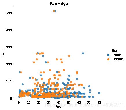
步骤6 绘制一个展示船票Fare, 与乘客年龄和性别的散点图
lm = sns.lmplot(x = 'Age', y = 'Fare', data = titanic, hue = 'Sex', fit_reg=False)
lm.set(title = 'Fare x Age')
axes = lm.axes
axes[0,0].set_ylim(-5,)
axes[0,0].set_xlim(-5,85)
步骤7 有多少人生还?
titanic.Survived.sum()
342
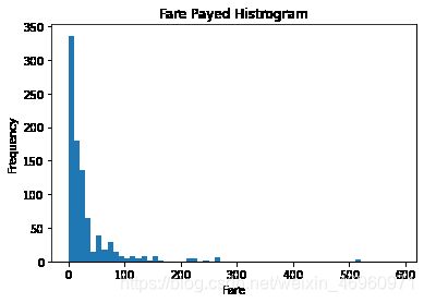
步骤8 绘制一个展示船票价格的直方图
df = titanic.Fare.sort_values(ascending = False)
df
binsVal = np.arange(0,600,10)
binsVal
plt.hist(df, bins = binsVal)
plt.xlabel('Fare')
plt.ylabel('Frequency')
plt.title('Fare Payed Histrogram')
plt.show()
练习8-创建数据框
探索Pokemon数据
步骤1 导入必要的库
import pandas as pd
步骤2 创建一个数据字典
raw_data = {"name": ['Bulbasaur', 'Charmander','Squirtle','Caterpie'],
            "evolution": ['Ivysaur','Charmeleon','Wartortle','Metapod'],
            "type": ['grass', 'fire', 'water', 'bug'],
            "hp": [45, 39, 44, 45],
            "pokedex": ['yes', 'no','yes','no']
            }
步骤3 将数据字典存为一个名叫pokemon的数据框中
pokemon = pd.DataFrame(raw_data)
pokemon.head()
|
evolution |
hp |
name |
pokedex |
type |
| 0 |
Ivysaur |
45 |
Bulbasaur |
yes |
grass |
| 1 |
Charmeleon |
39 |
Charmander |
no |
fire |
| 2 |
Wartortle |
44 |
Squirtle |
yes |
water |
| 3 |
Metapod |
45 |
Caterpie |
no |
bug |
步骤4 数据框的列排序是字母顺序,请重新修改为name, type, hp, evolution, pokedex这个顺序
pokemon = pokemon[['name', 'type', 'hp', 'evolution','pokedex']]
pokemon
|
name |
type |
hp |
evolution |
pokedex |
| 0 |
Bulbasaur |
grass |
45 |
Ivysaur |
yes |
| 1 |
Charmander |
fire |
39 |
Charmeleon |
no |
| 2 |
Squirtle |
water |
44 |
Wartortle |
yes |
| 3 |
Caterpie |
bug |
45 |
Metapod |
no |
步骤5 添加一个列place
pokemon['place'] = ['park','street','lake','forest']
pokemon
|
name |
type |
hp |
evolution |
pokedex |
place |
| 0 |
Bulbasaur |
grass |
45 |
Ivysaur |
yes |
park |
| 1 |
Charmander |
fire |
39 |
Charmeleon |
no |
street |
| 2 |
Squirtle |
water |
44 |
Wartortle |
yes |
lake |
| 3 |
Caterpie |
bug |
45 |
Metapod |
no |
forest |
步骤6 查看每个列的数据类型
pokemon.dtypes
name         object
type         object
hp            int64
evolution    object
pokedex      object
place        object
dtype: object
练习9-时间序列
探索Apple公司股价数据
步骤1 导入必要的库
import pandas as pd
import numpy as np
import matplotlib.pyplot as plt
%matplotlib inline
步骤2 数据集地址
path9 = './exercise_data/Apple_stock.csv'
步骤3 读取数据并存为一个名叫apple的数据框
apple = pd.read_csv(path9)
apple.head()
|
Date |
Open |
High |
Low |
Close |
Volume |
Adj Close |
| 0 |
2014-07-08 |
96.27 |
96.80 |
93.92 |
95.35 |
65130000 |
95.35 |
| 1 |
2014-07-07 |
94.14 |
95.99 |
94.10 |
95.97 |
56305400 |
95.97 |
| 2 |
2014-07-03 |
93.67 |
94.10 |
93.20 |
94.03 |
22891800 |
94.03 |
| 3 |
2014-07-02 |
93.87 |
94.06 |
93.09 |
93.48 |
28420900 |
93.48 |
| 4 |
2014-07-01 |
93.52 |
94.07 |
93.13 |
93.52 |
38170200 |
93.52 |
步骤4 查看每一列的数据类型
apple.dtypes
Date          object
Open         float64
High         float64
Low          float64
Close        float64
Volume         int64
Adj Close    float64
dtype: object
步骤5 将Date这个列转换为datetime类型
apple.Date = pd.to_datetime(apple.Date)
apple['Date'].head()
0   2014-07-08
1   2014-07-07
2   2014-07-03
3   2014-07-02
4   2014-07-01
Name: Date, dtype: datetime64[ns]
步骤6 将Date设置为索引
apple = apple.set_index('Date')
apple.head()
|
Open |
High |
Low |
Close |
Volume |
Adj Close |
| Date |
|
|
|
|
|
|
| 2014-07-08 |
96.27 |
96.80 |
93.92 |
95.35 |
65130000 |
95.35 |
| 2014-07-07 |
94.14 |
95.99 |
94.10 |
95.97 |
56305400 |
95.97 |
| 2014-07-03 |
93.67 |
94.10 |
93.20 |
94.03 |
22891800 |
94.03 |
| 2014-07-02 |
93.87 |
94.06 |
93.09 |
93.48 |
28420900 |
93.48 |
| 2014-07-01 |
93.52 |
94.07 |
93.13 |
93.52 |
38170200 |
93.52 |
步骤7 有重复的日期吗?
apple.index.is_unique
True
步骤8 将index设置为升序
apple.sort_index(ascending = True).head()
|
Open |
High |
Low |
Close |
Volume |
Adj Close |
| Date |
|
|
|
|
|
|
| 1980-12-12 |
28.75 |
28.87 |
28.75 |
28.75 |
117258400 |
0.45 |
| 1980-12-15 |
27.38 |
27.38 |
27.25 |
27.25 |
43971200 |
0.42 |
| 1980-12-16 |
25.37 |
25.37 |
25.25 |
25.25 |
26432000 |
0.39 |
| 1980-12-17 |
25.87 |
26.00 |
25.87 |
25.87 |
21610400 |
0.40 |
| 1980-12-18 |
26.63 |
26.75 |
26.63 |
26.63 |
18362400 |
0.41 |
步骤9 找到每个月的最后一个交易日(business day)
apple_month = apple.resample('BM').mean()
apple_month
|
Open |
High |
Low |
Close |
Volume |
Adj Close |
| Date |
|
|
|
|
|
|
| 1980-12-31 |
30.481538 |
30.567692 |
30.443077 |
30.443077 |
2.586252e+07 |
0.473077 |
| 1981-01-30 |
31.754762 |
31.826667 |
31.654762 |
31.654762 |
7.249867e+06 |
0.493810 |
| 1981-02-27 |
26.480000 |
26.572105 |
26.407895 |
26.407895 |
4.231832e+06 |
0.411053 |
| 1981-03-31 |
24.937727 |
25.016818 |
24.836364 |
24.836364 |
7.962691e+06 |
0.387727 |
| 1981-04-30 |
27.286667 |
27.368095 |
27.227143 |
27.227143 |
6.392000e+06 |
0.423333 |
| ... |
... |
... |
... |
... |
... |
... |
| 2014-03-31 |
533.593333 |
536.453810 |
530.070952 |
533.214286 |
5.954403e+07 |
75.750000 |
| 2014-04-30 |
540.081905 |
544.349048 |
536.262381 |
541.074286 |
7.660787e+07 |
76.867143 |
| 2014-05-30 |
601.301905 |
606.372857 |
598.332857 |
603.195714 |
6.828177e+07 |
86.058571 |
| 2014-06-30 |
222.360000 |
224.084286 |
220.735714 |
222.658095 |
5.745506e+07 |
91.885714 |
| 2014-07-31 |
94.294000 |
95.004000 |
93.488000 |
94.470000 |
4.218366e+07 |
94.470000 |
404 rows × 6 columns
步骤10 数据集中最早的日期和最晚的日期相差多少天?
(apple.index.max() - apple.index.min()).days
12261
步骤11 在数据中一共有多少个月?
apple_months = apple.resample('BM').mean()
len(apple_months.index)
404
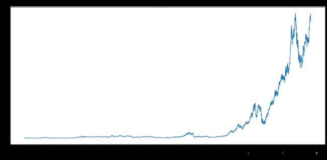
步骤12 按照时间顺序可视化Adj Close值
appl_open = apple['Adj Close'].plot(title = "Apple Stock")
fig = appl_open.get_figure()
fig.set_size_inches(13.5, 9)
练习10-删除数据
探索Iris纸鸢花数据
步骤1 导入必要的库
import pandas as pd
步骤2 数据集地址
path10 ='./exercise_data/iris.csv'
步骤3 将数据集存成变量iris
iris = pd.read_csv(path10)
iris.head()
|
5.1 |
3.5 |
1.4 |
0.2 |
Iris-setosa |
| 0 |
4.9 |
3.0 |
1.4 |
0.2 |
Iris-setosa |
| 1 |
4.7 |
3.2 |
1.3 |
0.2 |
Iris-setosa |
| 2 |
4.6 |
3.1 |
1.5 |
0.2 |
Iris-setosa |
| 3 |
5.0 |
3.6 |
1.4 |
0.2 |
Iris-setosa |
| 4 |
5.4 |
3.9 |
1.7 |
0.4 |
Iris-setosa |
步骤4 创建数据框的列名称
iris = pd.read_csv(path10,names = ['sepal_length','sepal_width', 'petal_length', 'petal_width', 'class'])
iris.head()
|
sepal_length |
sepal_width |
petal_length |
petal_width |
class |
| 0 |
5.1 |
3.5 |
1.4 |
0.2 |
Iris-setosa |
| 1 |
4.9 |
3.0 |
1.4 |
0.2 |
Iris-setosa |
| 2 |
4.7 |
3.2 |
1.3 |
0.2 |
Iris-setosa |
| 3 |
4.6 |
3.1 |
1.5 |
0.2 |
Iris-setosa |
| 4 |
5.0 |
3.6 |
1.4 |
0.2 |
Iris-setosa |
步骤5 数据框中有缺失值吗?
pd.isnull(iris).sum()
sepal_length    0
sepal_width     0
petal_length    0
petal_width     0
class           0
dtype: int64
步骤6 将列petal_length的第10到19行设置为缺失值
iris.iloc[10:20,2:3] = np.nan
iris.head(20)
|
sepal_length |
sepal_width |
petal_length |
petal_width |
class |
| 0 |
5.1 |
3.5 |
1.4 |
0.2 |
Iris-setosa |
| 1 |
4.9 |
3.0 |
1.4 |
0.2 |
Iris-setosa |
| 2 |
4.7 |
3.2 |
1.3 |
0.2 |
Iris-setosa |
| 3 |
4.6 |
3.1 |
1.5 |
0.2 |
Iris-setosa |
| 4 |
5.0 |
3.6 |
1.4 |
0.2 |
Iris-setosa |
| 5 |
5.4 |
3.9 |
1.7 |
0.4 |
Iris-setosa |
| 6 |
4.6 |
3.4 |
1.4 |
0.3 |
Iris-setosa |
| 7 |
5.0 |
3.4 |
1.5 |
0.2 |
Iris-setosa |
| 8 |
4.4 |
2.9 |
1.4 |
0.2 |
Iris-setosa |
| 9 |
4.9 |
3.1 |
1.5 |
0.1 |
Iris-setosa |
| 10 |
5.4 |
3.7 |
NaN |
0.2 |
Iris-setosa |
| 11 |
4.8 |
3.4 |
NaN |
0.2 |
Iris-setosa |
| 12 |
4.8 |
3.0 |
NaN |
0.1 |
Iris-setosa |
| 13 |
4.3 |
3.0 |
NaN |
0.1 |
Iris-setosa |
| 14 |
5.8 |
4.0 |
NaN |
0.2 |
Iris-setosa |
| 15 |
5.7 |
4.4 |
NaN |
0.4 |
Iris-setosa |
| 16 |
5.4 |
3.9 |
NaN |
0.4 |
Iris-setosa |
| 17 |
5.1 |
3.5 |
NaN |
0.3 |
Iris-setosa |
| 18 |
5.7 |
3.8 |
NaN |
0.3 |
Iris-setosa |
| 19 |
5.1 |
3.8 |
NaN |
0.3 |
Iris-setosa |
步骤7 将缺失值全部替换为1.0
iris.petal_length.fillna(1, inplace = True)
iris
|
sepal_length |
sepal_width |
petal_length |
petal_width |
class |
| 0 |
5.1 |
3.5 |
1.4 |
0.2 |
Iris-setosa |
| 1 |
4.9 |
3.0 |
1.4 |
0.2 |
Iris-setosa |
| 2 |
4.7 |
3.2 |
1.3 |
0.2 |
Iris-setosa |
| 3 |
4.6 |
3.1 |
1.5 |
0.2 |
Iris-setosa |
| 4 |
5.0 |
3.6 |
1.4 |
0.2 |
Iris-setosa |
| 5 |
5.4 |
3.9 |
1.7 |
0.4 |
Iris-setosa |
| 6 |
4.6 |
3.4 |
1.4 |
0.3 |
Iris-setosa |
| 7 |
5.0 |
3.4 |
1.5 |
0.2 |
Iris-setosa |
| 8 |
4.4 |
2.9 |
1.4 |
0.2 |
Iris-setosa |
| 9 |
4.9 |
3.1 |
1.5 |
0.1 |
Iris-setosa |
| 10 |
5.4 |
3.7 |
1.0 |
0.2 |
Iris-setosa |
| 11 |
4.8 |
3.4 |
1.0 |
0.2 |
Iris-setosa |
| 12 |
4.8 |
3.0 |
1.0 |
0.1 |
Iris-setosa |
| 13 |
4.3 |
3.0 |
1.0 |
0.1 |
Iris-setosa |
| 14 |
5.8 |
4.0 |
1.0 |
0.2 |
Iris-setosa |
| 15 |
5.7 |
4.4 |
1.0 |
0.4 |
Iris-setosa |
| 16 |
5.4 |
3.9 |
1.0 |
0.4 |
Iris-setosa |
| 17 |
5.1 |
3.5 |
1.0 |
0.3 |
Iris-setosa |
| 18 |
5.7 |
3.8 |
1.0 |
0.3 |
Iris-setosa |
| 19 |
5.1 |
3.8 |
1.0 |
0.3 |
Iris-setosa |
| 20 |
5.4 |
3.4 |
1.7 |
0.2 |
Iris-setosa |
| 21 |
5.1 |
3.7 |
1.5 |
0.4 |
Iris-setosa |
| 22 |
4.6 |
3.6 |
1.0 |
0.2 |
Iris-setosa |
| 23 |
5.1 |
3.3 |
1.7 |
0.5 |
Iris-setosa |
| 24 |
4.8 |
3.4 |
1.9 |
0.2 |
Iris-setosa |
| 25 |
5.0 |
3.0 |
1.6 |
0.2 |
Iris-setosa |
| 26 |
5.0 |
3.4 |
1.6 |
0.4 |
Iris-setosa |
| 27 |
5.2 |
3.5 |
1.5 |
0.2 |
Iris-setosa |
| 28 |
5.2 |
3.4 |
1.4 |
0.2 |
Iris-setosa |
| 29 |
4.7 |
3.2 |
1.6 |
0.2 |
Iris-setosa |
| ... |
... |
... |
... |
... |
... |
| 120 |
6.9 |
3.2 |
5.7 |
2.3 |
Iris-virginica |
| 121 |
5.6 |
2.8 |
4.9 |
2.0 |
Iris-virginica |
| 122 |
7.7 |
2.8 |
6.7 |
2.0 |
Iris-virginica |
| 123 |
6.3 |
2.7 |
4.9 |
1.8 |
Iris-virginica |
| 124 |
6.7 |
3.3 |
5.7 |
2.1 |
Iris-virginica |
| 125 |
7.2 |
3.2 |
6.0 |
1.8 |
Iris-virginica |
| 126 |
6.2 |
2.8 |
4.8 |
1.8 |
Iris-virginica |
| 127 |
6.1 |
3.0 |
4.9 |
1.8 |
Iris-virginica |
| 128 |
6.4 |
2.8 |
5.6 |
2.1 |
Iris-virginica |
| 129 |
7.2 |
3.0 |
5.8 |
1.6 |
Iris-virginica |
| 130 |
7.4 |
2.8 |
6.1 |
1.9 |
Iris-virginica |
| 131 |
7.9 |
3.8 |
6.4 |
2.0 |
Iris-virginica |
| 132 |
6.4 |
2.8 |
5.6 |
2.2 |
Iris-virginica |
| 133 |
6.3 |
2.8 |
5.1 |
1.5 |
Iris-virginica |
| 134 |
6.1 |
2.6 |
5.6 |
1.4 |
Iris-virginica |
| 135 |
7.7 |
3.0 |
6.1 |
2.3 |
Iris-virginica |
| 136 |
6.3 |
3.4 |
5.6 |
2.4 |
Iris-virginica |
| 137 |
6.4 |
3.1 |
5.5 |
1.8 |
Iris-virginica |
| 138 |
6.0 |
3.0 |
4.8 |
1.8 |
Iris-virginica |
| 139 |
6.9 |
3.1 |
5.4 |
2.1 |
Iris-virginica |
| 140 |
6.7 |
3.1 |
5.6 |
2.4 |
Iris-virginica |
| 141 |
6.9 |
3.1 |
5.1 |
2.3 |
Iris-virginica |
| 142 |
5.8 |
2.7 |
5.1 |
1.9 |
Iris-virginica |
| 143 |
6.8 |
3.2 |
5.9 |
2.3 |
Iris-virginica |
| 144 |
6.7 |
3.3 |
5.7 |
2.5 |
Iris-virginica |
| 145 |
6.7 |
3.0 |
5.2 |
2.3 |
Iris-virginica |
| 146 |
6.3 |
2.5 |
5.0 |
1.9 |
Iris-virginica |
| 147 |
6.5 |
3.0 |
5.2 |
2.0 |
Iris-virginica |
| 148 |
6.2 |
3.4 |
5.4 |
2.3 |
Iris-virginica |
| 149 |
5.9 |
3.0 |
5.1 |
1.8 |
Iris-virginica |
150 rows × 5 columns
步骤8 删除列class
del iris['class']
iris.head()
|
sepal_length |
sepal_width |
petal_length |
petal_width |
| 0 |
5.1 |
3.5 |
1.4 |
0.2 |
| 1 |
4.9 |
3.0 |
1.4 |
0.2 |
| 2 |
4.7 |
3.2 |
1.3 |
0.2 |
| 3 |
4.6 |
3.1 |
1.5 |
0.2 |
| 4 |
5.0 |
3.6 |
1.4 |
0.2 |
步骤9 将数据框前三行设置为缺失值
iris.iloc[0:3 ,:] = np.nan
iris.head()
|
sepal_length |
sepal_width |
petal_length |
petal_width |
| 0 |
NaN |
NaN |
NaN |
NaN |
| 1 |
NaN |
NaN |
NaN |
NaN |
| 2 |
NaN |
NaN |
NaN |
NaN |
| 3 |
4.6 |
3.1 |
1.5 |
0.2 |
| 4 |
5.0 |
3.6 |
1.4 |
0.2 |
步骤10 删除有缺失值的行
iris = iris.dropna(how='any')
iris.head()
|
sepal_length |
sepal_width |
petal_length |
petal_width |
| 3 |
4.6 |
3.1 |
1.5 |
0.2 |
| 4 |
5.0 |
3.6 |
1.4 |
0.2 |
| 5 |
5.4 |
3.9 |
1.7 |
0.4 |
| 6 |
4.6 |
3.4 |
1.4 |
0.3 |
| 7 |
5.0 |
3.4 |
1.5 |
0.2 |
步骤11 重新设置索引
iris = iris.reset_index(drop = True)
iris.head()
|
sepal_length |
sepal_width |
petal_length |
petal_width |
| 0 |
4.6 |
3.1 |
1.5 |
0.2 |
| 1 |
5.0 |
3.6 |
1.4 |
0.2 |
| 2 |
5.4 |
3.9 |
1.7 |
0.4 |
| 3 |
4.6 |
3.4 |
1.4 |
0.3 |
| 4 |
5.0 |
3.4 |
1.5 |
0.2 |