语音信号处理:librosa
1 librosa介绍
Librosa是一个用于音频和音乐分析的Python库,专为音乐信息检索(Music Information Retrieval,MIR)社区设计。自从2015年首次发布以来,Librosa已成为音频分析和处理领域中最受欢迎的工具之一。它提供了一套清晰、高效的函数来处理音频信号,并提取音乐和音频中的信息。

Librosa在音乐和音频分析方面提供了强大而灵活的工具,适用于从基础研究到实际应用的各个层面。它的广泛应用和强大功能使其成为音频分析领域的重要工具之一。与其他工具相比,Librosa存在如下优势:
-
易用性: Librosa的API设计简洁直观,便于快速上手和使用。
-
功能丰富: 提供了广泛的音频分析和处理功能。
-
灵活性: 可以轻松集成到更复杂的音频处理和机器学习流程中。
-
社区支持: 强大的社区支持确保了持续的发展和维护。
官网地址:https://librosa.org/doc/latest/index.html
1.1 核心特性
1.1.1 音频信号处理
-
读取和写入: Librosa支持读取和写入多种格式的音频文件,包括常见的WAV、MP3、FLAC等。
-
重采样: 支持对音频信号进行重采样,即改变音频的采样率。
1.1.2 音频特征提取
-
频谱特征: 包括短时傅里叶变换(STFT)、梅尔频谱(Mel-spectrogram)、色度频谱(Chromagram)等。
-
时域特征: 如零交叉率(Zero-Crossing Rate)、能量(RMS Energy)等。
1.1.3 音乐节拍和节奏分析
-
节拍跟踪: 自动检测音频中的节拍和节奏。
-
时序分段: 根据节奏将音乐分割成小段。
1.1.4 音高和音调检测
-
音高提取: 从音频信号中提取音高信息,用于旋律分析和音乐转录。
-
音调识别: 识别音频片段中的音调。
1.2 应用领域
1.2.1 音乐信息检索
-
音乐分类和标注: 根据音频特征将音乐自动分类,如流派、情感等。
-
音乐推荐系统: 根据音频分析提供个性化音乐推荐。
1.2.2 音频分析
-
语音处理: 在语音识别和语音合成中分析语音信号。
-
环境声音识别: 识别和分类环境中的各种声音。
1.2.3 音乐制作和编辑
-
自动音乐剪辑: 根据节奏和节拍自动剪辑音乐。
-
音乐可视化: 制作音乐的频谱可视化。
1.3 常用函数
-
load: 加载音频文件 -
stft: 短时傅里叶变换 -
istft: 短时傅里叶逆变换 -
magphase: 将STFT表示转换为幅度和相位表示 -
mel: 计算梅尔频率 -
melspectrogram: 计算梅尔频谱 -
mfcc: 计算MFCC系数 -
chroma_stft: 计算STFT表示的色度分布 -
onset_detect: 检测音频信号的起点 -
tempogram: 计算节奏图 -
beat_track: 通过节奏图确定节拍位置 -
cqt: 计算常量Q变换 -
cqt_hz_to_note: 将频率转换为音符 -
note_to_hz: 将音符转换为频率
2 librosa函数
2.1 Audio loading
| load(path, *[, sr, mono, offset, duration, ...]) |
Load an audio file as a floating point time series. |
| stream(path, *, block_length, frame_length, ...) |
Stream audio in fixed-length buffers. |
| to_mono(y) |
Convert an audio signal to mono by averaging samples across channels. |
| resample(y, *, orig_sr, target_sr[, ...]) |
Resample a time series from orig_sr to target_sr |
| get_duration(*[, y, sr, S, n_fft, ...]) |
Compute the duration (in seconds) of an audio time series, feature matrix, or filename. |
| get_samplerate(path) |
Get the sampling rate for a given fil |
2.2 Time-domain processing
| autocorrelate(y, *[, max_size, axis]) |
Bounded-lag auto-correlation |
| lpc(y, *, order[, axis]) |
Linear Prediction Coefficients via Burg's method |
| zero_crossings(y, *[, threshold, ...]) |
Find the zero-crossings of a signal |
| mu_compress(x, *[, mu, quantize]) |
mu-law compression |
| mu_expand(x, *[, mu, quantize]) |
mu-law expansion |
2.3 Signal generation
| clicks(*[, times, frames, sr, hop_length, ...]) |
Construct a "click track". |
| tone(frequency, *[, sr, length, duration, phi]) |
Construct a pure tone (cosine) signal at a given frequency. |
| chirp(*, fmin, fmax[, sr, length, duration, ...]) |
Construct a "chirp" or "sine-sweep" signal. |
2.4 Spectral representations
| stft(y, *[, n_fft, hop_length, win_length, ...]) |
Short-time Fourier transform (STFT). |
| istft(stft_matrix, *[, hop_length, ...]) |
Inverse short-time Fourier transform (ISTFT). |
| reassigned_spectrogram(y, *[, sr, S, n_fft, ...]) |
Time-frequency reassigned spectrogram. |
| cqt(y, *[, sr, hop_length, fmin, n_bins, ...]) |
Compute the constant-Q transform of an audio signal. |
| icqt(C, *[, sr, hop_length, fmin, ...]) |
Compute the inverse constant-Q transform. |
| hydrid_cqt(y, *[, sr, hop_length, fmin, ...]) |
Compute the hybrid constant-Q transform of an audio signal. |
| pseudo_cqt(y, *[, sr, hop_length, fmin, ...]) |
Compute the pseudo constant-Q transform of an audio signal. |
| vqt(y, *[, sr, hop_length, fmin, n_bins, ...]) |
Compute the variable-Q transform of an audio signal. |
| iirt(y, *[, sr, win_length, hop_length, ...]) |
Time-frequency representation using IIR filters |
| fmt(y, *[, t_min, n_fmt, kind, beta, ...]) |
Fast Mellin transform (FMT) |
| magphase(D, *[, power]) |
Separate a complex-valued spectrogram D into its magnitude (S) and phase (P) components, so that |
2.5 Phase recovery
| griffinlim(S, *[, n_iter, hop_length, ...]) |
Approximate magnitude spectrogram inversion using the "fast" Griffin-Lim algorithm. |
| griffinlim_cqt(C, *[, n_iter, sr, ...]) |
Approximate constant-Q magnitude spectrogram inversion using the "fast" Griffin-Lim algorithm. |
2.6 Harmonics
| interp_harmonics(x, *, freqs, harmonics[, ...]) |
Compute the energy at harmonics of time-frequency representation. |
| salience(S, *, freqs, harmonics[, weights, ...]) |
Harmonic salience function. |
| f0_harmonics(x, *, f0, freqs, harmonics[, ...]) |
Compute the energy at selected harmonics of a time-varying fundamental frequency. |
| phase_vocoder(D, *, rate[, hop_length, n_fft]) |
Phase vocoder. |
2.7 Magnitude scaling
| amplitude_to_db(S, *[, ref, amin, top_db]) |
Convert an amplitude spectrogram to dB-scaled spectrogram. |
| db_to_amplitude(S_db, *[, ref]) |
Convert a dB-scaled spectrogram to an amplitude spectrogram. |
| power_to_db(S, *[, ref, amin, top_db]) |
Convert a power spectrogram (amplitude squared) to decibel (dB) units |
| db_to_power(S_db, *[, ref]) |
Convert a dB-scale spectrogram to a power spectrogram. |
| perceptual_weighting(S, frequencies, *[, kind]) |
Perceptual weighting of a power spectrogram. |
| frequency_weighting(frequencies, *[, kind]) |
Compute the weighting of a set of frequencies. |
| multi_frequency_weighting( frequencies, *[, ...]) |
Compute multiple weightings of a set of frequencies. |
| A_weighting(frequencies, *[, min_db]) |
Compute the A-weighting of a set of frequencies. |
| B_weighting(frequencies, *[, min_db]) |
Compute the B-weighting of a set of frequencies. |
| C_weighting(frequencies, *[, min_db]) |
Compute the C-weighting of a set of frequencies. |
| D_weighting(frequencies, *[, min_db]) |
Compute the D-weighting of a set of frequencies. |
| pcen(S, *[, sr, hop_length, gain, bias, ...]) |
Per-channel energy normalization (PCEN) |
2.8 Time unit conversion
| frames_to_samples(frames, *[, hop_length, n_fft]) |
Convert frame indices to audio sample indices. |
| frames_to_time(frames, *[, sr, hop_length, ...]) |
Convert frame counts to time (seconds). |
| samples_to_frames(samples, *[, hop_length, ...]) |
Convert sample indices into STFT frames. |
| samples_to_time(samples, *[, sr]) |
Convert sample indices to time (in seconds). |
| time_to_frames(times, *[, sr, hop_length, n_fft]) |
Convert time stamps into STFT frames. |
| time_to_samples(times, *[, sr]) |
Convert timestamps (in seconds) to sample indices. |
| blocks_to_frames(blocks, *, block_length) |
Convert block indices to frame indices |
| blocks_to_samples(blocks, *, block_length, ...) |
Convert block indices to sample indices |
| blocks_to_time(blocks, *, block_length, ...) |
Convert block indices to time (in seconds) |
2.9 Frequency unit conversion
| hz_to_note(frequencies, **kwargs) |
Convert one or more frequencies (in Hz) to the nearest note names. |
| hz_to_midi(frequencies) |
Get MIDI note number(s) for given frequencies |
| hz_to_svara_h(frequencies, *, Sa[, abbr, ...]) |
Convert frequencies (in Hz) to Hindustani svara |
| hz_to_svara_c(frequencies, *, Sa, mela[, ...]) |
Convert frequencies (in Hz) to Carnatic svara |
| hz_to_fjs(frequencies, *[, fmin, unison, ...]) |
Convert one or more frequencies (in Hz) from a just intonation scale to notes in FJS notation. |
| midi_to_hz(notes) |
Get the frequency (Hz) of MIDI note(s) |
| midi_to_note(midi, *[, octave, cents, key, ...]) |
Convert one or more MIDI numbers to note strings. |
| midi_to_svara_h(midi, *, Sa[, abbr, octave, ...]) |
Convert MIDI numbers to Hindustani svara |
| midi_to_svara_c(midi, *, Sa, mela[, abbr, ...]) |
Convert MIDI numbers to Carnatic svara within a given melakarta raga |
| note_to_hz(note, **kwargs) |
Convert one or more note names to frequency (Hz) |
| note_to_midi(note, *[, round_midi]) |
Convert one or more spelled notes to MIDI number(s). |
| note_to_svara_h(notes, *, Sa[, abbr, ...]) |
Convert western notes to Hindustani svara |
| note_to_svara_c(notes, *, Sa, mela[, abbr, ...]) |
Convert western notes to Carnatic svara |
| hz_to_mel(frequencies, *[, htk]) |
Convert Hz to Mels |
| hz_to_octs(frequencies, *[, tuning, ...]) |
Convert frequencies (Hz) to (fractional) octave numbers. |
| mel_to_hz(mels, *[, htk]) |
Convert mel bin numbers to frequencies |
| octs_to_hz(octs, *[, tuning, bins_per_octave]) |
Convert octaves numbers to frequencies. |
| A4_to_tuning(A4, *[, bins_per_octave]) |
Convert a reference pitch frequency (e.g., |
| tuning_to_A4(tuning, *[, bins_per_octave]) |
Convert a tuning deviation (from 0) in fractions of a bin per octave (e.g., |
2.8 Music notation
| key_to_notes(key, *[, unicode]) |
List all 12 note names in the chromatic scale, as spelled according to a given key (major or minor). |
| key_to_degress(key) |
Construct the diatonic scale degrees for a given key. |
| mela_to_svara(mela, *[, abbr, unicode]) |
Spell the Carnatic svara names for a given melakarta raga |
| mela_to_degress(mela) |
Construct the svara indices (degrees) for a given melakarta raga |
| thaat_to_degress(thaat) |
Construct the svara indices (degrees) for a given thaat |
| list_mela() |
List melakarta ragas by name and index. |
| list_thaat() |
List supported thaats by name. |
| fifths_to_node(*, unison, fifths[, unicode]) |
Calculate the note name for a given number of perfect fifths from a specified unison. |
| interval_to_fjs(interval, *[, unison, ...]) |
Convert an interval to Functional Just System (FJS) notation. |
| interval_frequencies(n_bins, *, fmin, intervals) |
Construct a set of frequencies from an interval set |
| pythagorean_intervals(*[, bins_per_octave, ...]) |
Pythagorean intervals |
| plimit_intervals(*, primes[, ...]) |
Construct p-limit intervals for a given set of prime factors. |
2.9 Frequency range generation
| fft_frequencies(*[, sr, n_fft]) |
Alternative implementation of np.fft.fftfreq |
| cqt_frequencies(n_bins, *, fmin[, ...]) |
Compute the center frequencies of Constant-Q bins. |
| mel_frequencies([n_mels, fmin, fmax, htk]) |
Compute an array of acoustic frequencies tuned to the mel scale. |
| tempo_frequencies(n_bins, *[, hop_length, sr]) |
Compute the frequencies (in beats per minute) corresponding to an onset auto-correlation or tempogram matrix. |
| fourier_tempo_frequencies(*[, sr, ...]) |
Compute the frequencies (in beats per minute) corresponding to a Fourier tempogram matrix. |
2.10 Pitch and tuning
| pyin(y, *, fmin, fmax[, sr, frame_length, ...]) |
Fundamental frequency (F0) estimation using probabilistic YIN (pYIN). |
| yin(y, *, fmin, fmax[, sr, frame_length, ...]) |
Fundamental frequency (F0) estimation using the YIN algorithm. |
| estimate_tuning(*[, y, sr, S, n_fft, ...]) |
Estimate the tuning of an audio time series or spectrogram input. |
| pitch_tuning(frequencies, *[, resolution, ...]) |
Given a collection of pitches, estimate its tuning offset (in fractions of a bin) relative to A440=440.0Hz. |
| piptrack(*[, y, sr, S, n_fft, hop_length, ...]) |
Pitch tracking on thresholded parabolically-interpolated STFT. |
2.11 Miscellaneous
| samples_like(X, *[, hop_length, n_fft, axis]) |
Return an array of sample indices to match the time axis from a feature matrix. |
| times_like(X, *[, sr, hop_length, n_fft, axis]) |
Return an array of time values to match the time axis from a feature matrix. |
| get_fftlib() |
Get the FFT library currently used by librosa |
| set_fftlib([lib]) |
Set the FFT library used by librosa. |
3 librosa使用
3.1 librosa安装
pip install librosa3.2 加载音频文件
函数原型:
librosa.load(path, sr=22050, mono=True, offset=0.0, duration=None)读取音频文件,默认采样率是22050,如果要保留音频的原始采样率,使用sr = None。
参数:
path :音频文件的路径。
sr :采样率,如果为“None”使用音频自身的采样率
mono :bool,是否将信号转换为单声道
offset :float,在此时间之后开始阅读(以秒为单位)
持续时间:float,仅加载这么多的音频(以秒为单位)
返回:
y :音频时间序列
sr :音频的采样率
-
librosa.load 函数返回的时间序列是一个一维数组,表示音频信号在时间轴上的采样值。在 librosa中,时间轴的方向是沿着数组的第一个轴,即 axis=0。
-
因此,数组的每个元素代表了时间轴上的一个采样点。 例如,如果采样率为22050Hz,那么每秒会有 22050 个采样点,我们可以将其理解为在时间轴上每隔1/22050秒就采集一次音频信号的值。
-
因此,如果音频的长度为T秒,那么librosa.load函数返回的时间序列就是一个长度为T×sr的一维数组,其中sr是采样率。
-
需要注意的是,返回的时间序列并不一定是归一化的,也不一定是整数类型。在后续的处理中,我们通常需要对其进行归一化、类型转换等操作。
import librosa

audio_data = '../data/mel001.wav'
data, sr = librosa.load(audio_data)
print('采样率:', sr)
print('数据长度:', data.shape)
print('数据:', data)
运行代码显示:
采样率: 22050
数据长度: (4879296,)
数据: [0. 0. 0. ... 0. 0. 0.]
3.3 重采样
函数原型:
librosa.resample(y, orig_sr, target_sr, fix=True, scale=False)重新采样从orig_sr到target_sr的时间序列
参数:
y :音频时间序列。可以是单声道或立体声。
orig_sr :y的原始采样率
target_sr :目标采样率
fix:bool,调整重采样信号的长度,使其大小恰好为len(y)/orig_sr*target_sr=t∗target_sr
scale:bool,缩放重新采样的信号,以使y和y_hat具有大约相等的总能量。
返回:
y_hat :重采样之后的音频数组
示例代码:
import librosa

audio_data = '../data/mel001.wav'
data, sr = librosa.load(audio_data)

y_hat = librosa.resample(data, orig_sr=22050, target_sr=44100)
print('原始数据长度:', data.shape)
print('重采样后数据长度:', y_hat.shape)
运行代码显示:
原始数据长度: (4879296,)
重采样后数据长度: (9758592,)
3.4 读取时长
函数原型:
librosa.get_duration(y=None, sr=22050, S=None, n_fft=2048, hop_length=512, center=True, filename=None)计算时间序列的的持续时间(以秒为单位)
参数:
y :音频时间序列
sr :y的音频采样率
S :STFT矩阵或任何STFT衍生的矩阵(例如,色谱图或梅尔频谱图)。根据频谱图输入计算的持续时间仅在达到帧分辨率之前才是准确的。如果需要高精度,则最好直接使用音频时间序列。
n_fft :S的 FFT窗口大小
hop_length :S列之间的音频样本数
center :布尔值
如果为True,则S [:, t]的中心为y [t * hop_length]
如果为False,则S [:, t]从y[t * hop_length]开始
filename :如果提供,则所有其他参数都将被忽略,并且持续时间是直接从音频文件中计算得出的。
返回:
d :持续时间(以秒为单位)
示例代码:
import librosa

audio_data = '../data/mel001.wav'
data, sr = librosa.load(audio_data)
y_hat = librosa.resample(data, orig_sr=22050, target_sr=44100)
duration1 = librosa.get_duration(y=data)
duration2 = librosa.get_duration(y=y_hat, sr=44100)
print('原始时长:', duration1)
print('重采样后时长:', duration2)
运行代码显示:
原始时长: 221.28326530612244
重采样后时长: 221.28326530612244
3.5 读取采样率
函数原型:
librosa.get_samplerate(path)参数:
path :音频文件的路径
返回:音频文件的采样率
示例代码:
import librosa

audio_data = '../data/mel001.wav'
sr = librosa.get_samplerate(audio_data)
print('采样率:', sr)
运行代码显示:
采样率: 441003.6 写音频
函数原型:
librosa.output.write_wav(path, y, sr, norm=False)将时间序列输出为.wav文件
参数:
path:保存输出wav文件的路径
y :音频时间序列。
sr :y的采样率
norm:bool,是否启用幅度归一化。将数据缩放到[-1,+1]范围。
在0.8.0以后的版本,librosa这个函数已经删除,推荐用下面的函数:
import soundfile
soundfile.write(file, data, samplerate)
参数:
file:保存输出wav文件的路径
data:音频数据
samplerate:采样率
示例代码:
import librosa
import soundfile

audio_data = '../data/mel001.wav'
data, sr = librosa.load(audio_data)
y_hat = librosa.resample(data, orig_sr=22050, target_sr=44100)
soundfile.write('../data/re_mel001.wav', data, 44100)
3.7 过零率
函数原型:
librosa.feature.zero_crossing_rate(y, frame_length = 2048, hop_length = 512, center = True) 计算音频时间序列的过零率。
参数:
y :音频时间序列
frame_length :帧长
hop_length :帧移
center:bool,如果为True,则通过填充y的边缘来使帧居中。
返回:
zcr:zcr[0,i]是第i帧中的过零率
示例代码:
import librosa

audio_data = '../data/mel001.wav'
data, sr = librosa.load(audio_data, sr=44100)
print(librosa.feature.zero_crossing_rate(data))
print(data.shape)
运行代码显示:
[[0. 0. 0. ... 0. 0. 0.]]
(9758592,)
3.8 波形图
函数原型:
librosa.display.waveshow(y,*,sr=22050,max_points=11025,x_axis="time",offset=0.0,marker="",where="post",label=None,ax=None,**kwargs,)绘制波形的幅度包络线
参数:
y :音频时间序列
sr :y的采样率
x_axis :str {‘time’,‘off’,‘none’}或None,如果为“时间”,则在x轴上给定时间刻度线。
offset:水平偏移(以秒为单位)开始波形图
示例代码:
import librosa
import librosa.display
import matplotlib.pyplot as plt

y, sr = librosa.load('../data/mel001.wav', duration=20)
librosa.display.waveshow(y, sr=sr)
plt.show()
运行代码显示:

3.9 短时傅里叶变换
librosa.stft(y, n_fft=2048, hop_length=None, win_length=None, window='hann', center=True, pad_mode='reflect')短时傅立叶变换(STFT),返回一个复数矩阵D(F,T)
参数:
y:音频时间序列
n_fft:FFT窗口大小,n_fft=hop_length+overlapping
hop_length:帧移,如果未指定,则默认win_length/4。
win_length:每一帧音频都由window()加窗。窗长win_length,然后用零填充以匹配N_FFT。默认win_length=n_fft。
window:字符串,元组,数字,函数 shape =(n_fft, )
窗口(字符串,元组或数字);
窗函数,例如scipy.signal.hanning
长度为n_fft的向量或数组
center:bool
如果为True,则填充信号y,以使帧 D [:, t]以y [t * hop_length]为中心。
如果为False,则D [:, t]从y [t * hop_length]开始
dtype:D的复数值类型。默认值为64-bit complex复数
pad_mode:如果center = True,则在信号的边缘使用填充模式。默认情况下,STFT使用reflection padding。
返回:
STFT矩阵,shape =(1 + n(fft)/2,t)

3.10 幅值和相位
函数原型:
librosa.magphase(D, power=1)librosa提供了专门将复数矩阵D(F, T)分离为幅值S和相位P的函数,D = S * P
参数:
- D:经过stft得到的复数矩阵
- power:幅度谱的指数,例如,1代表能量,2代表功率,等等。
返回:
- D_mag:幅值D,
- D_phase:相位P,
phase = exp(1.j * phi),phi是复数矩阵的相位角np.angle(D)
3.11 短时傅里叶逆变换
函数原型:
librosa.istft(stft_matrix, hop_length=None, win_length=None, window='hann', center=True, length=None)短时傅立叶逆变换(ISTFT),将复数值D(f,t)频谱矩阵转换为时间序列y,窗函数、帧移等参数应与stft相同
参数:
stft_matrix :经过STFT之后的矩阵
hop_length :帧移,默认为
win_length :窗长,默认为n_fft
window:字符串,元组,数字,函数或shape = (n_fft, )
窗口(字符串,元组或数字)
窗函数,例如scipy.signal.hanning
长度为n_fft的向量或数组
center:bool
如果为True,则假定D具有居中的帧
如果False,则假定D具有左对齐的帧
length:如果提供,则输出y为零填充或剪裁为精确长度音频
返回:
y :时域信号
3.12 功率转dB
函数原型
librosa.core.power_to_db(S, ref=1.0)将功率谱(幅值平方)转换为dB单位,与这个函数相反的是 librosa.db_to_power(S)
参数:
S:输入功率
ref :参考值,振幅abs(S)相对于ref进行缩放
返回:
dB为单位的S,
示例代码:
import librosa
import librosa.display
import numpy as np
import matplotlib.pyplot as plt

y, sr = librosa.load('../data/mel001.wav')
S = np.abs(librosa.stft(y))     # 幅值
print(librosa.power_to_db(S ** 2))
plt.figure()
plt.subplot(2, 1, 1)
librosa.display.specshow(S ** 2, sr=sr, y_axis='log')  # 绘制功率谱
plt.colorbar()
plt.title('Power spectrogram')
plt.subplot(2, 1, 2)
# 相对于峰值功率计算dB, 那么其他的dB都是负的,注意看后边cmp值
librosa.display.specshow(librosa.power_to_db(S ** 2, ref=np.max), sr=sr, y_axis='log', x_axis='time')   # 绘制对数功率谱
plt.colorbar(format='%+2.0f dB')
plt.title('Log-Power spectrogram')
plt.set_cmap("autumn")
plt.tight_layout()
plt.show()
运行代码显示:
[[-35.042385 -35.042385 -35.042385 ... -35.042385 -35.042385 -35.042385]
 [-35.042385 -35.042385 -35.042385 ... -35.042385 -35.042385 -35.042385]
 [-35.042385 -35.042385 -35.042385 ... -35.042385 -35.042385 -35.042385]
 ...
 [-35.042385 -35.042385 -35.042385 ... -35.042385 -35.042385 -35.042385]
 [-35.042385 -35.042385 -35.042385 ... -35.042385 -35.042385 -35.042385]
 [-35.042385 -35.042385 -35.042385 ... -35.042385 -35.042385 -35.042385]]
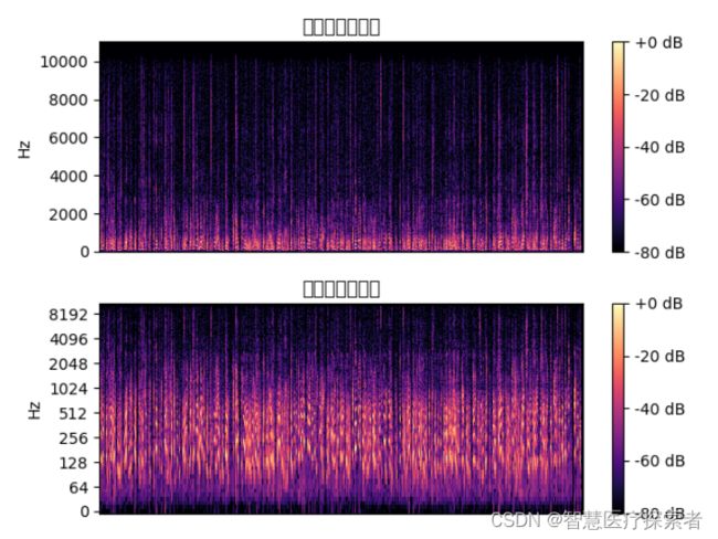
3.13 绘制频谱图
librosa.display.specshow(data, x_axis=None, y_axis=None, sr=22050, hop_length=512)参数:
data:要显示的矩阵
sr :采样率
hop_length :帧移
x_axis 、y_axis :x和y轴的范围
频率类型
‘linear’,‘fft’,‘hz’:频率范围由FFT窗口和采样率确定
‘log’:频谱以对数刻度显示
‘mel’:频率由mel标度决定
时间类型
time:标记以毫秒,秒,分钟或小时显示。值以秒为单位绘制。
s:标记显示为秒。
ms:标记以毫秒为单位显示。
所有频率类型均以Hz为单位绘制
import librosa
import librosa.display
import numpy as np
import matplotlib.pyplot as plt

y, sr = librosa.load('../data/mel001.wav')
plt.figure()

D = librosa.amplitude_to_db(np.abs(librosa.stft(y)), ref=np.max)
plt.subplot(2, 1, 1)
librosa.display.specshow(D, y_axis='linear')
plt.colorbar(format='%+2.0f dB')
plt.title('线性频率功率谱')

plt.subplot(2, 1, 2)
librosa.display.specshow(D, y_axis='log')
plt.colorbar(format='%+2.0f dB')
plt.title('对数频率功率谱')
plt.show()
运行代码显示:
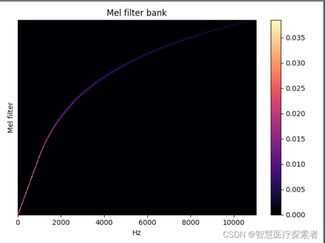
3.14 Mel滤波器组
librosa.filters.mel(sr, n_fft, n_mels=128, fmin=0.0, fmax=None, htk=False, norm=1)创建一个滤波器组矩阵以将FFT合并成Mel频率
参数:
sr :输入信号的采样率
n_fft :FFT组件数
n_mels :产生的梅尔带数
fmin :最低频率(Hz)
fmax:最高频率(以Hz为单位)。如果为None,则使用fmax = sr / 2.0
norm:{None,1,np.inf} [标量]
如果为1,则将三角mel权重除以mel带的宽度(区域归一化)。否则,保留所有三角形的峰值为1.0
返回:
Mel变换矩阵
import librosa
import librosa.display
import matplotlib.pyplot as plt

melfb = librosa.filters.mel(sr=22050, n_fft=2048)
plt.figure()
librosa.display.specshow(melfb, x_axis='linear')
plt.ylabel('Mel filter')
plt.title('Mel filter bank')
plt.colorbar()
plt.tight_layout()
plt.show()
运行代码显示:
3.15 计算Mel频谱
librosa.feature.melspectrogram(y=None, sr=22050, S=None, n_fft=2048, hop_length=512, win_length=None, window='hann', center=True, pad_mode='reflect', power=2.0)如果提供了频谱图输入S,则通过mel_f.dot(S)将其直接映射到mel_f上。如果提供了时间序列输入y,sr,则首先计算其幅值频谱S,然后通过mel_f.dot(S ** power)将其映射到mel scale上 。默认情况下,power= 2在功率谱上运行。
参数:
y :音频时间序列
sr :采样率
S :频谱
n_fft :FFT窗口的长度
hop_length :帧移
win_length :窗口的长度为win_length,默认win_length = n_fft
window :字符串,元组,数字,函数或shape =(n_fft, )
窗口规范(字符串,元组或数字);看到scipy.signal.get_window
窗口函数,例如 scipy.signal.hanning
长度为n_fft的向量或数组
center:bool
如果为True,则填充信号y,以使帧 t以y [t * hop_length]为中心。
如果为False,则帧t从y [t * hop_length]开始
power:幅度谱的指数。例如1代表能量,2代表功率,等等
n_mels:滤波器组的个数 1288
fmax:最高频率
返回:
Mel频谱shape=(n_mels, t)
import librosa
import librosa.display
import numpy as np
import matplotlib.pyplot as plt

y, sr = librosa.load('../data/mel001.wav')
# 方法一:使用时间序列求Mel频谱
print(librosa.feature.melspectrogram(y=y, sr=sr))

# 方法二:使用stft频谱求Mel频谱
D = np.abs(librosa.stft(y)) ** 2  # stft频谱
S = librosa.feature.melspectrogram(S=D)  # 使用stft频谱求Mel频谱

plt.figure(figsize=(10, 4))
librosa.display.specshow(librosa.power_to_db(S, ref=np.max), y_axis='mel', fmax=8000, x_axis='time')
plt.colorbar(format='%+2.0f dB')
plt.title('Mel spectrogram')
plt.tight_layout()
plt.show()
运行代码显示:
[[0. 0. 0. ... 0. 0. 0.]
 [0. 0. 0. ... 0. 0. 0.]
 [0. 0. 0. ... 0. 0. 0.]
 ...
 [0. 0. 0. ... 0. 0. 0.]
 [0. 0. 0. ... 0. 0. 0.]
 [0. 0. 0. ... 0. 0. 0.]]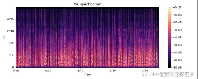
3.16 提取Log-Mel Spectrogram特征
Log-Mel Spectrogram特征是目前在语音识别和环境声音识别中很常用的一个特征,由于CNN在处理图像上展现了强大的能力,使得音频信号的频谱图特征的使用愈加广泛,甚至比MFCC使用的更多。在librosa中,Log-Mel Spectrogram特征的提取只需几行代码:
import librosa

y, sr = librosa.load('../data/mel001.wav', sr=16000)

# 提取 mel spectrogram feature
melspec = librosa.feature.melspectrogram(y=y, sr=sr, n_fft=1024, hop_length=512, n_mels=128)

# 转换到对数刻度
logmelspec = librosa.power_to_db(melspec)
print(logmelspec.shape)
运行代码显示:
(128, 6916)可见,Log-Mel Spectrogram特征是二维数组的形式,128表示Mel频率的维度(频域),64为时间帧长度(时域),所以Log-Mel Spectrogram特征是音频信号的时频表示特征。其中,n_fft指的是窗的大小,这里为1024;hop_length表示相邻窗之间的距离,这里为512,也就是相邻窗之间有50%的overlap;n_mels为mel bands的数量,这里设为128。
3.17 提取MFCC系数
MFCC特征是一种在自动语音识别和说话人识别中广泛使用的特征。在librosa中,提取MFCC特征只需要一个函数:
librosa.feature.mfcc(y=None, sr=22050, S=None, n_mfcc=20, dct_type=2, norm='ortho', **kwargs)参数:
y:音频数据
sr:采样率
S:np.ndarray,对数功能梅尔谱图
n_mfcc:int>0,要返回的MFCC数量
dct_type:None, or {1, 2, 3} 离散余弦变换(DCT)类型。默认情况下,使用DCT类型2。
norm: None or ‘ortho’ 规范。如果dct_type为2或3,则设置norm =’ortho’使用正交DCT基础。 标准化不支持dct_type = 1。
返回:
M: MFCC序列
import librosa

y, sr = librosa.load('../data/mel001.wav', sr=16000)

# 提取 MFCC feature
mfccs = librosa.feature.mfcc(y=y, sr=sr, n_mfcc=40)
print(mfccs.shape)
运行代码显示:
(40, 6916)线性谱、梅尔谱、对数谱:经过FFT变换后得到语音数据的线性谱,对线性谱取Mel系数,得到梅尔谱;对线性谱取对数,得到对数谱。