计算机视觉python--SIFT算法
文章目录
- 1 sift的特征简介
-
- 1.1 SIFT算法可以解决的问题
- 1.2 SIFT算法实现步骤简述
- 2 关键点检测的相关概念
-
- 2.1 哪些点是SIFT中要查找的关键点(特征点)
- 2.2 什么是尺度空间
- 2.3 高斯模糊
- 2.4 高斯金字塔
- 2.5 DOG局部极值检测
-
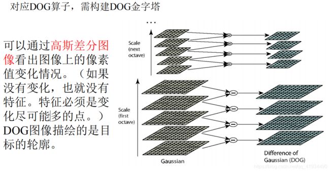
- 2.5.1 DoG高斯差分金字塔
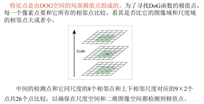
- 2.5.2 DoG的局部极值点
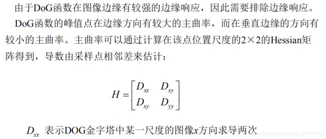
- 2.5.3 去除边缘响应
- 3 关键点
-
- 3.1 关键点的方向匹配
- 3.2 关键点描述
- 3.3 关键点匹配
- 4 代码实现
-
- 4.1 关键点检测
- 4.2 描述子匹配
- 4.3 实现数据集中查找匹配数高的图片
- 5 分析与结论
- 6 匹配地理标记图像
-
- 6.1 实验代码
- 6.2 实验结果
- 6.3 实验结果分析
- 6.4 实验遇到的问题
- 7 RANSAC算法筛选SIFT特征匹配
-
- 7.1 RANSAC算法简介
- 7.2 RANSAC算法原理
- 7.3 RANSAC算法流程在SIFT特征筛选中的主要流程
- 7.4 代码实现
- 7.6 实验分析
1 sift的特征简介
1.1 SIFT算法可以解决的问题
• 目标的旋转、缩放、平移(RST)
• 图像仿射/投影变换(视点viewpoint)
• 弱光照影响(illumination)
• 部分目标遮挡(occlusion)
• 杂物场景(clutter)
• 噪声
1.2 SIFT算法实现步骤简述
SIFT算法的实质可以归为在不同尺度空间上查找特征点(关键点)的问题。
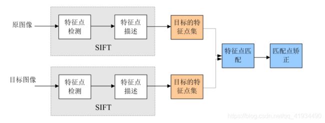
SIFT算法实现特征匹配主要有三个流程,1、提取关键点;2、对关键点附加 详细的信息(局部特征),即描述符;3、通过特征点(附带上特征向量的关 键点)的两两比较找出相互匹配的若干对特征点,建立景物间的对应关系。
2 关键点检测的相关概念
2.1 哪些点是SIFT中要查找的关键点(特征点)
这些点是一些十分突出的点不会因光照、尺度、旋转等因素的改变而消 失,比如角点、边缘点、暗区域的亮点以及亮区域的暗点。既然两幅图像中 有相同的景物,那么使用某种方法分别提取各自的稳定点,这些点之间会有 相互对应的匹配点
2.2 什么是尺度空间
关键点检测的相关概念 尺度空间中各尺度图像的 模糊程度逐渐变大,能够模拟 人在距离目标由近到远时目标 在视网膜上的形成过程。 尺度越大图像越模糊。
根据文献《Scale-space theory: A basic tool for analysing structures at different scales》可知,高斯核是唯一可以产生 多尺度空间的核,一个 图像的尺度空间,L(x, y, σ) ,定义为原始图像 I(x, y)与一个可变尺度的2 维高斯函数G(x, y, σ) 卷积运算。
2.3 高斯模糊

2.4 高斯金字塔
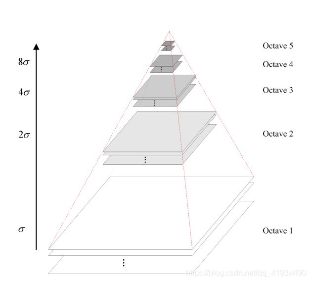
高斯金子塔的构建过程可分为两步: (1)对图像做高斯平滑; (2)对图像做降采样。 为了让尺度体现其连续性,在简单 下采样的基础上加上了高斯滤波。 一幅图像可以产生几组(octave) 图像,一组图像包括几层 (interval)图像
高斯图像金字塔共o组、s层, 则有: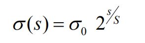 ——尺度空间坐标; s——sub-level层坐标; σ0——初始尺度; S——每组层数(一般为3~5)
最后可将组内和组间尺度 归为: 
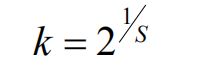
i——金字塔组数 n——每一组的层数
2.5 DOG局部极值检测

2.5.1 DoG高斯差分金字塔
2.5.2 DoG的局部极值点
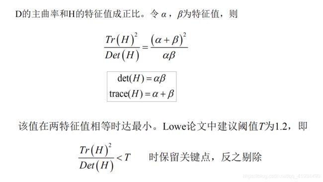
2.5.3 去除边缘响应
3 关键点
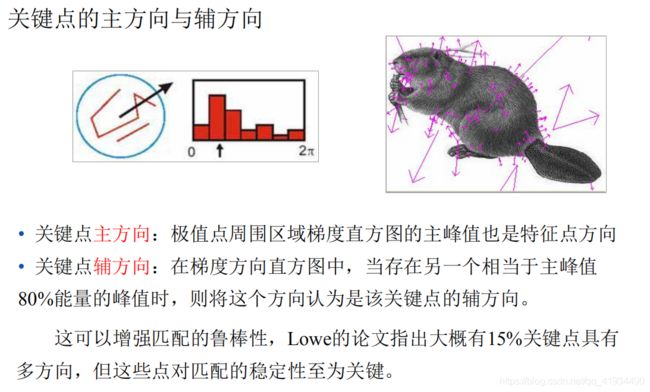
3.1 关键点的方向匹配

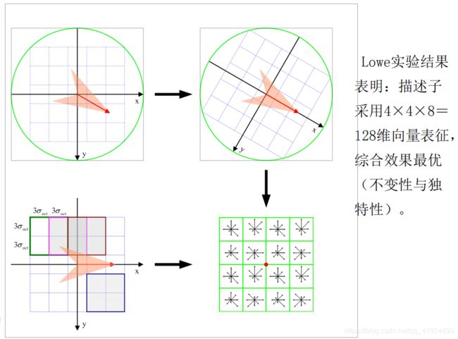
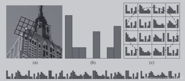
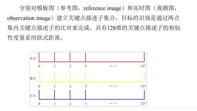
3.2 关键点描述

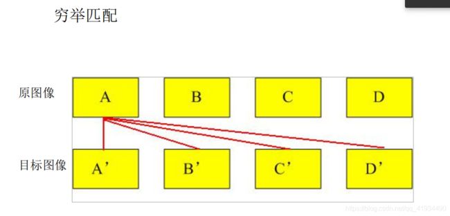
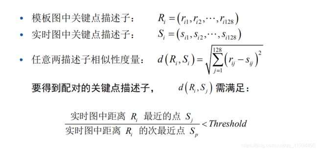
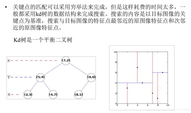
3.3 关键点匹配
4 代码实现
4.1 关键点检测
# -*- coding: utf-8 -*-
from PIL import Image
from pylab import *
from PCV.localdescriptors import sift
from PCV.localdescriptors import harris

# 添加中文字体支持
from matplotlib.font_manager import FontProperties
font = FontProperties(fname=r"c:\windows\fonts\SimSun.ttc", size=14)

imname = 'd:/picture/002/1.png'
im = array(Image.open(imname).convert('L'))
sift.process_image(imname, 'empire.sift')
l1, d1 = sift.read_features_from_file('empire.sift')

figure()
gray()
subplot(131)
sift.plot_features(im, l1, circle=False)
title(u'SIFT特征',fontproperties=font)
subplot(132)
sift.plot_features(im, l1, circle=True)
title(u'用圆圈表示SIFT特征尺度',fontproperties=font)

# 检测harris角点
harrisim = harris.compute_harris_response(im)

subplot(133)
filtered_coords = harris.get_harris_points(harrisim, 6, 0.1)
imshow(im)
plot([p[1] for p in filtered_coords], [p[0] for p in filtered_coords], '+c')
axis('off')
title(u'Harris角点',fontproperties=font)

show()


sift 的特征会比图片运行出来的harris角点要多 表明特征是包括角点 、边缘点、暗区域的亮点以及亮区域的暗点
4.2 描述子匹配
from PIL import Image
from pylab import *
import sys
from PCV.localdescriptors import sift


if len(sys.argv) >= 3:
  im1f, im2f = sys.argv[1], sys.argv[2]
else:
#  im1f = '../data/sf_view1.jpg'
#  im2f = '../data/sf_view2.jpg'
  im1f = '../data/crans_1_small.jpg'
  im2f = '../data/crans_2_small.jpg'
#  im1f = '../data/climbing_1_small.jpg'
#  im2f = '../data/climbing_2_small.jpg'
im1 = array(Image.open(im1f))
im2 = array(Image.open(im2f))

sift.process_image(im1f, 'out_sift_1.txt')
l1, d1 = sift.read_features_from_file('out_sift_1.txt')
figure()
gray()
subplot(121)
sift.plot_features(im1, l1, circle=False)

sift.process_image(im2f, 'out_sift_2.txt')
l2, d2 = sift.read_features_from_file('out_sift_2.txt')
subplot(122)
sift.plot_features(im2, l2, circle=False)

#matches = sift.match(d1, d2)
matches = sift.match_twosided(d1, d2)
print '{} matches'.format(len(matches.nonzero()[0]))

figure()
gray()
sift.plot_matches(im1, im2, l1, l2, matches, show_below=True)
show()
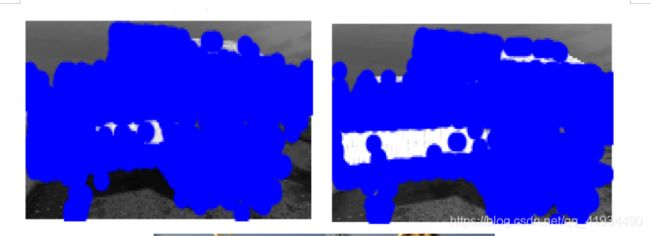

这边发现了问题 就是图片的像素较高的话会出现错误
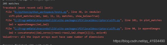
虽然能够计算match 但是无法显示连线图
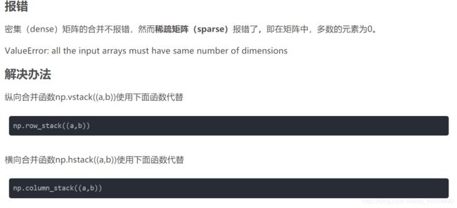
下面是百度到的解决办法
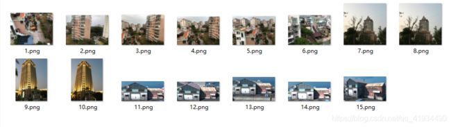
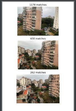
4.3 实现数据集中查找匹配数高的图片
from PIL import Image
from pylab import *
from PCV.localdescriptors import sift
import matplotlib.pyplot as plt # plt 用于显示图片


im1f = 'd:/picture/002/1.png'
im1 = array(Image.open(im1f))
sift.process_image(im1f, 'out_sift_1.txt')
l1, d1 = sift.read_features_from_file('out_sift_1.txt')

arr=[]#单维链表数组
arrHash = {}#字典型数组
for i in range(2,7):
    im2f = 'd:/picture/002/'+str(i)+'.png'
    im2 = array(Image.open(im2f))
    sift.process_image(im2f, 'out_sift_2.txt')
    l2, d2 = sift.read_features_from_file('out_sift_2.txt')
    matches = sift.match_twosided(d1, d2)
    length=len(matches.nonzero()[0])
    length=int(length)
    arr.append(length)#添加新的值
    arrHash[length]=im2f#添加新的值

arr.sort()#数组排序
arr=arr[::-1]#数组反转
arr=arr[:5]#截取数组元素到第五个
i=0
plt.figure(figsize=(5,12))#设置输出图像的大小
for item in arr:
    if(arrHash.get(item)!=None):
        img=arrHash.get(item)
        im1 = array(Image.open(img))
        ax=plt.subplot(511 + i)#设置子团位置
        ax.set_title('{} matches'.format(item))#设置子图标题
        plt.axis('off')#不显示坐标轴
        imshow(im1)
        i = i + 1

plt.show()
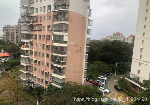
输入图片
5 分析与结论
由实验结果可看出,SIFT点的特点为
1.视角和旋转变化不变性
2.光照不变性
3.尺度不变性
但是在实验过程中发现对模糊的图像和边缘平滑的图像,检测出的特征点过少,对圆更是无能为力
6 匹配地理标记图像
6.1 实验代码
# -*- coding: utf-8 -*-
from pylab import *
from PIL import Image
from PCV.localdescriptors import sift
from PCV.tools import imtools
import pydot

""" This is the example graph illustration of matching images from Figure 2-10.
To download the images, see ch2_download_panoramio.py."""

#download_path = "panoimages"  # set this to the path where you downloaded the panoramio images
#path = "/FULLPATH/panoimages/"  # path to save thumbnails (pydot needs the full system path)

download_path = "d:/picture/002/"  # set this to the path where you downloaded the panoramio images
path = "d:/picture/002/"  # path to save thumbnails (pydot needs the full system path)

# list of downloaded filenames
imlist = imtools.get_imlist(download_path)
nbr_images = len(imlist)

# extract features
featlist = [imname[:-3] + 'sift' for imname in imlist]
for i, imname in enumerate(imlist):
    sift.process_image(imname, featlist[i])

matchscores = zeros((nbr_images, nbr_images))

for i in range(nbr_images):
    for j in range(i, nbr_images):  # only compute upper triangle
        print ('comparing ', imlist[i], imlist[j])
        l1, d1 = sift.read_features_from_file(featlist[i])
        l2, d2 = sift.read_features_from_file(featlist[j])
        matches = sift.match_twosided(d1, d2)
        nbr_matches = sum(matches > 0)
        print ('number of matches = ', nbr_matches)
        matchscores[i, j] = nbr_matches
print ("The match scores is: \n", matchscores)

# copy values
for i in range(nbr_images):
    for j in range(i + 1, nbr_images):  # no need to copy diagonal
        matchscores[j, i] = matchscores[i, j]

#可视化

threshold = 2  # min number of matches needed to create link

g = pydot.Dot(graph_type='graph')  # don't want the default directed graph

for i in range(nbr_images):
    for j in range(i + 1, nbr_images):
        if matchscores[i, j] > threshold:
            # first image in pair
            im = Image.open(imlist[i])
            im.thumbnail((100, 100))
            filename = path + str(i) + '.png'
            im.save(filename)  # need temporary files of the right size
            g.add_node(pydot.Node(str(i), fontcolor='transparent', shape='rectangle', image=filename))

            # second image in pair
            im = Image.open(imlist[j])
            im.thumbnail((100, 100))
            filename = path + str(j) + '.png'
            im.save(filename)  # need temporary files of the right size
            g.add_node(pydot.Node(str(j), fontcolor='transparent', shape='rectangle', image=filename))

            g.add_edge(pydot.Edge(str(i), str(j)))
g.write_png('whitehouse.png')
6.2 实验结果

6.3 实验结果分析
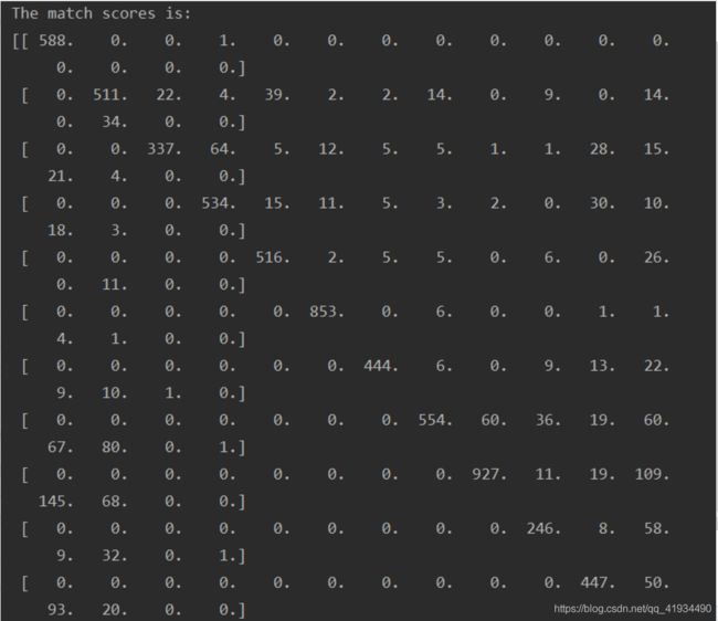
实验结果出来是矩阵 矩阵中最大的数是和自己的匹配 其他的非零的数字都代表着一条连线 因为我采用的图片具有较高的分辨度 所以分成了四组彼此没有出现干扰的线 而当出现干扰的线也就是有较小匹配度的时候怎么不让线出现呢 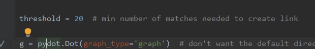
修改threshould 越大线越少 也就是限制匹配度
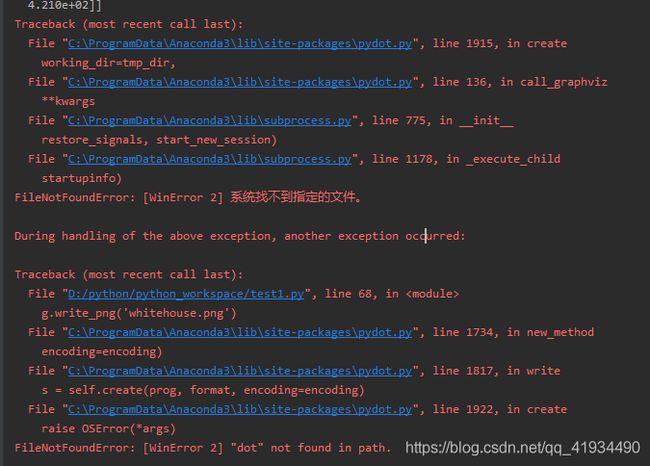
6.4 实验遇到的问题

没有安装pydot
安装pydot的步骤如下
先下载Graphviz:graphviz-2.38.msi
将安装路径 c:\Program Files (x86)\Graphviz2.38\bin 添加到path中
再用cmd 运行pip install graphviz 安装
接着pip install pydot 安装
![]()
这个问题是因为![]()
只支持处理.jpg的文件 把图片后缀修改下就行
这个问题根据百度是因为安装graphviz的时候用了pip install 来安装 但是我卸载了再用 Anaconda来安装 conda install 来安装但是问题依然不能解决。网上还有个办法是将本来的pydot文件下的self.prog=‘dot’改为’dot.exe’ 但还是没办法解决问题。
哦哦哦解决了 再代码中添加
就可以运行了
7 RANSAC算法筛选SIFT特征匹配
7.1 RANSAC算法简介
RANSAC(RANdom SAmple Consensus)随机抽样一致算法,是一种在包含离群点在内的数据集里,通过迭代的方式估计模型的参数。举个例子,我们计算单应性矩阵时,初始匹配有很多的误匹配即是一个有离群点的数据集,然后我们估计出单应性矩阵。
RANSAC是一种算法的思路,在计算机视觉中应用较多。它是一种不确定的算法,即有一定的概率得出一个合理的结果,当然也会出现错误的结果。如果要提高概率,一个要提高迭代的次数,在一个就是减少数据集离群点的比例。
RANSAC 在视觉中有很多的应用,比如2D特征点匹配,3D点云匹配,在图片或者点云中识别直线,识别可以参数化的形状。RANSAC还可以用来拟合函数等。
7.2 RANSAC算法原理
OpenCV中滤除误匹配对采用RANSAC算法寻找一个最佳单应性矩阵H,矩阵大小为3×3。RANSAC目的是找到最优的参数矩阵使得满足该矩阵的数据点个数最多,通常令h33=1来归一化矩阵。由于单应性矩阵有8个未知参数,至少需要8个线性方程求解,对应到点位置信息上,一组点对可以列出两个方程,则至少包含4组匹配点对。

RANSAC算法从匹配数据集中随机抽出4个样本并保证这4个样本之间不共线,计算出单应性矩阵,然后利用这个模型测试所有数据,并计算满足这个模型数据点的个数与投影误差(即代价函数),若此模型为最优模型,则对应的代价函数最小。

7.3 RANSAC算法流程在SIFT特征筛选中的主要流程
RANSAC算法在SIFT特征筛选中的主要流程是:
(1) 从样本集中随机抽选一个RANSAC样本,即4个匹配点对
(2) 根据这4个匹配点对计算变换矩阵M
(3) 根据样本集,变换矩阵M,和误差度量函数计算满足当前变换矩阵的一致集consensus,并返回一致集中元素个数
(4) 根据当前一致集中元素个数判断是否最优(最大)一致集,若是则更新当前最优一致集
(5) 更新当前错误概率p,若p大于允许的最小错误概率则重复(1)至(4)继续迭代,直到当前错误概率p小于最小错误概率
7.4 代码实现
# -*- coding: utf-8 -*-
import cv2
import numpy as np
import random

def compute_fundamental(x1, x2):
    n = x1.shape[1]
    if x2.shape[1] != n:
        raise ValueError("Number of points don't match.")

    # build matrix for equations
    A = np.zeros((n, 9))
    for i in range(n):
        A[i] = [x1[0, i] * x2[0, i], x1[0, i] * x2[1, i], x1[0, i] * x2[2, i],
                x1[1, i] * x2[0, i], x1[1, i] * x2[1, i], x1[1, i] * x2[2, i],
                x1[2, i] * x2[0, i], x1[2, i] * x2[1, i], x1[2, i] * x2[2, i]]

    # compute linear least square solution
    U, S, V = np.linalg.svd(A)
    F = V[-1].reshape(3, 3)

    # constrain F
    # make rank 2 by zeroing out last singular value
    U, S, V = np.linalg.svd(F)
    S[2] = 0
    F = np.dot(U, np.dot(np.diag(S), V))

    return F / F[2, 2]


def compute_fundamental_normalized(x1, x2):
    """    Computes the fundamental matrix from corresponding points
        (x1,x2 3*n arrays) using the normalized 8 point algorithm. """

    n = x1.shape[1]
    if x2.shape[1] != n:
        raise ValueError("Number of points don't match.")

    # normalize image coordinates
    x1 = x1 / x1[2]
    mean_1 = np.mean(x1[:2], axis=1)
    S1 = np.sqrt(2) / np.std(x1[:2])
    T1 = np.array([[S1, 0, -S1 * mean_1[0]], [0, S1, -S1 * mean_1[1]], [0, 0, 1]])
    x1 = np.dot(T1, x1)

    x2 = x2 / x2[2]
    mean_2 = np.mean(x2[:2], axis=1)
    S2 = np.sqrt(2) / np.std(x2[:2])
    T2 = np.array([[S2, 0, -S2 * mean_2[0]], [0, S2, -S2 * mean_2[1]], [0, 0, 1]])
    x2 = np.dot(T2, x2)

    # compute F with the normalized coordinates
    F = compute_fundamental(x1, x2)
    # print (F)
    # reverse normalization
    F = np.dot(T1.T, np.dot(F, T2))

    return F / F[2, 2]

def randSeed(good, num = 8):
    '''
    :param good: 初始的匹配点对
    :param num: 选择随机选取的点对数量
    :return: 8个点对list
    '''
    eight_point = random.sample(good, num)
    return eight_point

def PointCoordinates(eight_points, keypoints1, keypoints2):
    '''
    :param eight_points: 随机八点
    :param keypoints1: 点坐标
    :param keypoints2: 点坐标
    :return:8个点
    '''
    x1 = []
    x2 = []
    tuple_dim = (1.,)
    for i in eight_points:
        tuple_x1 = keypoints1[i[0].queryIdx].pt + tuple_dim
        tuple_x2 = keypoints2[i[0].trainIdx].pt + tuple_dim
        x1.append(tuple_x1)
        x2.append(tuple_x2)
    return np.array(x1, dtype=float), np.array(x2, dtype=float)


def ransac(good, keypoints1, keypoints2, confidence,iter_num):
    Max_num = 0
    good_F = np.zeros([3,3])
    inlier_points = []
    for i in range(iter_num):
        eight_points = randSeed(good)
        x1,x2 = PointCoordinates(eight_points, keypoints1, keypoints2)
        F = compute_fundamental_normalized(x1.T, x2.T)
        num, ransac_good = inlier(F, good, keypoints1, keypoints2, confidence)
        if num > Max_num:
            Max_num = num
            good_F = F
            inlier_points = ransac_good
    print(Max_num, good_F)
    return Max_num, good_F, inlier_points


def computeReprojError(x1, x2, F):
    """
    计算投影误差
    """
    ww = 1.0/(F[2,0]*x1[0]+F[2,1]*x1[1]+F[2,2])
    dx = (F[0,0]*x1[0]+F[0,1]*x1[1]+F[0,2])*ww - x2[0]
    dy = (F[1,0]*x1[0]+F[1,1]*x1[1]+F[1,2])*ww - x2[1]
    return dx*dx + dy*dy

def inlier(F,good, keypoints1,keypoints2,confidence):
    num = 0
    ransac_good = []
    x1, x2 = PointCoordinates(good, keypoints1, keypoints2)
    for i in range(len(x2)):
        line = F.dot(x1[i].T)
        #在对极几何中极线表达式为[A B C],Ax+By+C=0,  方向向量可以表示为[-B,A]
        line_v = np.array([-line[1], line[0]])
        err = h = np.linalg.norm(np.cross(x2[i,:2], line_v)/np.linalg.norm(line_v))
        # err = computeReprojError(x1[i], x2[i], F)
        if abs(err) < confidence:
            ransac_good.append(good[i])
            num += 1
    return num, ransac_good


if __name__ =='__main__':
    im1 = 'd:/picture/004/1.jpg'
    im2 = 'd:/picture/004/2.jpg'

    print(cv2.__version__)
    psd_img_1 = cv2.imread(im1, cv2.IMREAD_COLOR)
    psd_img_2 = cv2.imread(im2, cv2.IMREAD_COLOR)
    # 3) SIFT特征计算
    sift = cv2.xfeatures2d.SIFT_create()
    # find the keypoints and descriptors with SIFT
    kp1, des1 = sift.detectAndCompute(psd_img_1, None)
    kp2, des2 = sift.detectAndCompute(psd_img_2, None)

    # FLANN 参数设计
    match = cv2.BFMatcher()
    matches = match.knnMatch(des1, des2, k=2)

    # Apply ratio test
    # 比值测试,首先获取与 A距离最近的点 B (最近)和 C (次近),
    # 只有当 B/C 小于阀值时(0.75)才被认为是匹配,
    # 因为假设匹配是一一对应的,真正的匹配的理想距离为0
    good = []
    for m, n in matches:
        if m.distance < 0.75 * n.distance:
            good.append([m])
    print(good[0][0])

    print("number of feature points:",len(kp1), len(kp2))
    print(type(kp1[good[0][0].queryIdx].pt))
    print("good match num:{} good match points:".format(len(good)))
    for i in good:
        print(i[0].queryIdx, i[0].trainIdx)


    Max_num, good_F, inlier_points = ransac(good, kp1, kp2, confidence=30, iter_num=500)
    # cv2.drawMatchesKnn expects list of lists as matches.
    # img3 = np.ndarray([2, 2])
    # img3 = cv2.drawMatchesKnn(img1, kp1, img2, kp2, good[:10], img3, flags=2)

    # cv2.drawMatchesKnn expects list of lists as matches.

    img3 = cv2.drawMatchesKnn(psd_img_1,kp1,psd_img_2,kp2,good,None,flags=2)
    img4 = cv2.drawMatchesKnn(psd_img_1,kp1,psd_img_2,kp2,inlier_points,None,flags=2)
    cv2.namedWindow('image1', cv2.WINDOW_NORMAL)
    cv2.namedWindow('image2', cv2.WINDOW_NORMAL)
    cv2.imshow("image1",img3)
    cv2.imshow("image2",img4)
    cv2.waitKey(0)#等待按键按下
    cv2.destroyAllWindows()#清除所有窗口
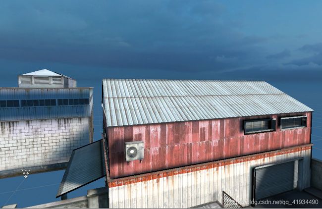
景深丰富
原图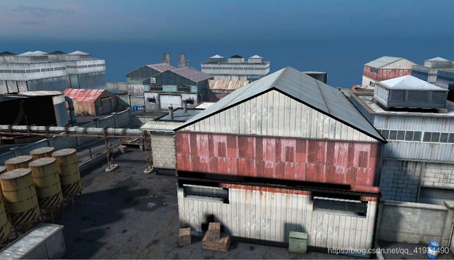

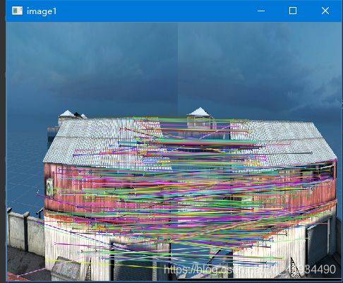
剔除前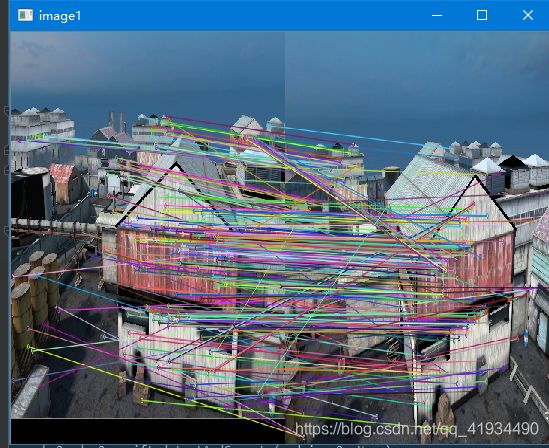
景色单一
原图

剔除前
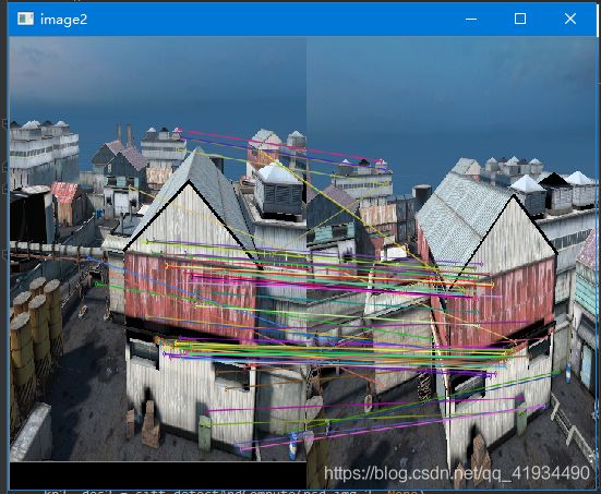
剔除后

7.6 实验分析
1.景深复杂的图片特征匹配点较多, 匹配线较为密集,因此我们主要观察图片下方的匹配线。可以看到,使用RANSAC算法后可以将很多不匹配的点删去,由图可见效果很好,但是因为误差的存在依旧残留一些错误的匹配点。
2.景色单一的图片再后面的剔除中会把一些原本就是正确的匹配点给剔除掉,由此可见该算法还存在着一些问题