yolov5 评价指标

相信刚上手yolov5的小伙伴，对train.py和val.py 中的评价指标很疑惑吧。

今天为大家讲解一下，争取用朴素的语言讲明白。

1.混淆矩阵（confusion matrix)

文字解释：

简单来说是判断这个类分的正确不正确的。那这个判断是不是有4种情况。

（1） 真实值是正确的，预测值也是正确的。称为TP

（2） 真实值是错误的，但是预测值是错误的。称为TN

（3） 真实值是正确的，预测值是错误的。称为FN

（4） 真实值是错误的，预测值是正确的。称为FP

这个也很好和英文名对应，真实值与预测值一致的话就是T，代表True。不一致就是F，代表False。如果预测值为负的，就是N，代表Negative。如果预测值为正，就是P，代表Positive。

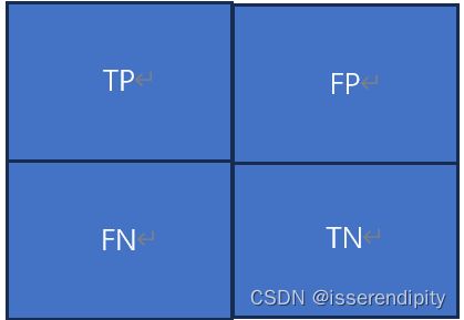
这样子站位，横坐标为True，即真实值。纵坐标为Predict，即预测值。当TP和TN越大越好，分类效果越好。

下面几个公式很重要哦（一般来说，positive就是我们预测的指标哦）

 （1）召回率：真实值为正确的时候，召回了多少正确预测值也正确的概率。

（2）精确率度：预测与真实一样时，要求的评价指标正确的概率。

（3）准确度：预测值与真实值一致时，占所有样本的概率。

 以上三个当然是越高越好。一般yolov5给出的混淆矩阵都是经过归一化 的。看对角线的值越大越好。

代码解释：

官方文档为：kaanakan/object_detection_confusion_matrix: Python class for calculating confusion matrix for object detection task (github.com)

 我们主要讲解yolov5中有关混淆矩阵的代码

在val.py中，一共三次调用了confusion_matrix函数。

第一次调用：

confusion_matrix = ConfusionMatrix(nc=nc)

 接着进入ConfusionMatrix类中，构造这个类，并初始化。

class ConfusionMatrix:
    # Updated version of https://github.com/kaanakan/object_detection_confusion_matrix
    def __init__(self, nc, conf=0.25, iou_thres=0.45):
        self.matrix = np.zeros((nc + 1, nc + 1))
        self.nc = nc  # number of classes
        self.conf = conf
        self.iou_thres = iou_thres

 第二次调用：

if plots:
                    confusion_matrix.process_batch(predn, labelsn)

 plots为run 的参数，本为ture。调用ConfusionMatrix类中的process_batch函数。

    def process_batch(self, detections, labels):  #detections为预测的框，labels为真实的框
        """
        Return intersection-over-union (Jaccard index) of boxes.
        Both sets of boxes are expected to be in (x1, y1, x2, y2) format.
        Arguments:
            detections (Array[N, 6]), x1, y1, x2, y2, conf, class
            labels (Array[M, 5]), class, x1, y1, x2, y2
        Returns:
            None, updates confusion matrix accordingly
        """
        detections = detections[detections[:, 4] > self.conf]  # 如果预测框的之置信度大于设置的置信度，即上面初始化的置信度conf=0.25，时，保留这个预测框
        gt_classes = labels[:, 0].int()   # 获取真实框
        detection_classes = detections[:, 5].int()   #获取第几类标签
        iou = box_iou(labels[:, 1:], detections[:, :4])    #两者交叉的面积

        x = torch.where(iou > self.iou_thres)   #相交的面积大于0.45
        if x[0].shape[0]:
            matches = torch.cat((torch.stack(x, 1), iou[x[0], x[1]][:, None]), 1).cpu().numpy()
            if x[0].shape[0] > 1:  #获取最大阈值下的预测框
                matches = matches[matches[:, 2].argsort()[::-1]]
                matches = matches[np.unique(matches[:, 1], return_index=True)[1]]
                matches = matches[matches[:, 2].argsort()[::-1]]
                matches = matches[np.unique(matches[:, 0], return_index=True)[1]]
        else:
            matches = np.zeros((0, 3))

        n = matches.shape[0] > 0   # 满足条件的iou是否大于0个 bool
        m0, m1, _ = matches.transpose().astype(np.int16)  #m0为真实正样本框的索引值，m1时预测正样本索引值
        for i, gc in enumerate(gt_classes):
            j = m0 == i
            if n and sum(j) == 1:  # 简而言之，真实框预测到了。但是不一定分对了类,为TP+FP
                self.matrix[detection_classes[m1[j]], gc] += 1  # correct
            else:
                self.matrix[self.nc, gc] += 1  # background FP  没预测到，成为了背景板

        if n:
            for i, dc in enumerate(detection_classes):
                if not any(m1 == i):
                    self.matrix[dc, self.nc] += 1  # background FN  背景板加1

 第三次调用：

    if plots:
        confusion_matrix.plot(save_dir=save_dir, names=list(names.values()))
        callbacks.run('on_val_end')

 这个是显示混淆矩阵的。

    def plot(self, normalize=True, save_dir='', names=()):
        try:
            import seaborn as sn

            array = self.matrix / ((self.matrix.sum(0).reshape(1, -1) + 1E-6) if normalize else 1)  # normalize columns
            array[array < 0.005] = np.nan  # don't annotate (would appear as 0.00)

            fig = plt.figure(figsize=(12, 9), tight_layout=True)
            sn.set(font_scale=1.0 if self.nc < 50 else 0.8)  # for label size
            labels = (0 < len(names) < 99) and len(names) == self.nc  # apply names to ticklabels
            with warnings.catch_warnings():
                warnings.simplefilter('ignore')  # suppress empty matrix RuntimeWarning: All-NaN slice encountered
                sn.heatmap(array, annot=self.nc < 30, annot_kws={"size": 8}, cmap='Blues', fmt='.2f', square=True,
                           xticklabels=names + ['background FP'] if labels else "auto",
                           yticklabels=names + ['background FN'] if labels else "auto").set_facecolor((1, 1, 1))
            fig.axes[0].set_xlabel('True')
            fig.axes[0].set_ylabel('Predicted')
            fig.savefig(Path(save_dir) / 'confusion_matrix.png', dpi=250)
            plt.close()
        except Exception as e:
            print(f'WARNING: ConfusionMatrix plot failure: {e}')

 具体代码原理：先归一化后画图，具体代码我们就不看了。

 部分代码参考：【YOLOV5-5.x 源码解读】metrics.py_yolov5 metrics.py_满船清梦压星河HK的博客-CSDN博客

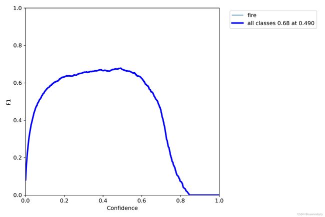
2.F1-score（保存在F1-curve)

当想要同时控制风险 ( recall ) 和成本 ( precision )怎么办？那就用 F1 Score 。

 

F1分数与置信度（x轴）之间的关系。F1分数是分类的一个衡量标准，是精确率和召回率的调和平均函数，介于0，1之间。越大越好。

 3.P-curve图

表示准确率与置信度的关系图线，横坐标置信度。

由下图可以看出置信度越高，准确率越高。

4.PR-curve

PR曲线中的P代表的是precision（精准率），R代表的是recall（召回率），其代表的是精准率与召回率的关系。

其中越接近（1，1）效果越好。

5.R-curve

召回率与置信度之间关系。

为什么置信度为0的时候，召回率一般不为1。

因为看召回率的公式，分母还有一个FN，还有可能判断为负样本。

置信程度越大，样本越接近真实目标，所以越接近（1，1）越好。

[email protected]&&mAP@[0.5:0.95]

AP（average precision )：平均精度。虽然叫平均精度，但是代表着对一个类精度的判断。而且也不是对precision求平均，是计算PR图中PR线与坐标轴的面积。如果一个模型的AP越大，也就是说PR曲线与坐标轴围成的面积越大，Precision与Recall在整体上也相对较高。

mPA（mean of average precision）:对所有类别的AP求平均值。AP反映的是对一个精度的判断，MPA反映对所有类精度的判断，当然越接近1越好啦。平时我们说的，某一目标检测算法的准确率达到了多少，这个准确率就泛指mAP。

想要解释后面两个就不得不提到IOU了。

iou：是交叉比，预测时预测框和真实标签框的交集比上并集。iou值越大说明预测的越准确。取值在【0,1】之间。

下面这个图可以形象化展示怎么计算的。

[email protected]：就是说mPA在iou>=0.5时计算的。也就是说，iou小于0.5时认为是负样本，不能判断出这个类别。大于0.5时才能画框展示出来类别。自然也是越大越好了。

mAP@[0.5:0.95]：是多个IOU阈值下的mAP，会在区间[0.5,0.95]内，以0.05为步长，取10个IOU阈值，分别计算这10个IOU阈值下的mAP，再取平均值。mAP@[0.5:0.95]越大，表示预测框越精准，因为它取到了更多IOU阈值大的情况。
部分参考：YOLO 模型的评估指标——IOU、Precision、Recall、F1-score、mAP_yolo评价指标_G.E.N.的博客-CSDN博客

 8.下面我们来看具体代码怎么实现以上几个图的：

在val.py中先初始化这几个参数。

    s = ('%20s' + '%11s' * 6) % ('Class', 'Images', 'Labels', 'P', 'R', '[email protected]', '[email protected]:.95')
    dt, p, r, f1, mp, mr, map50, map = [0.0, 0.0, 0.0], 0.0, 0.0, 0.0, 0.0, 0.0, 0.0, 0.0  #初始化

然后后面使用：

    if len(stats) and stats[0].any():
        p, r, ap, f1, ap_class = ap_per_class(*stats, plot=plots, save_dir=save_dir, names=names)  #Plot precision-recall curve at [email protected]
        ap50, ap = ap[:, 0], ap.mean(1)  # [email protected], [email protected]:0.95
        mp, mr, map50, map = p.mean(), r.mean(), ap50.mean(), ap.mean()
        nt = np.bincount(stats[3].astype(np.int64), minlength=nc) 

我们进到ap_per_class函数中看看：

#tp:整个数据集所有图片中所有预测框在每一个iou条件下(0.5~0.95)10个是否是TP
# conf:整个数据集所有图片的所有预测框的置信度
# pred_cls:预测类别
# plot:是否演示
def ap_per_class(tp, conf, pred_cls, target_cls, plot=False, save_dir='.', names=()):  
    """ Compute the average precision, given the recall and precision curves.
    Source: https://github.com/rafaelpadilla/Object-Detection-Metrics.
    # Arguments
        tp:  True positives (nparray, nx1 or nx10).
        conf:  Objectness value from 0-1 (nparray).
        pred_cls:  Predicted object classes (nparray).
        target_cls:  True object classes (nparray).
        plot:  Plot precision-recall curve at [email protected]
        save_dir:  Plot save directory
    # Returns
        The average precision as computed in py-faster-rcnn.
    """
    # 计算mAP 需要将tp按照conf降序排列
    # Sort by objectness  按conf从大到小排序 返回数据对应的索引
    i = np.argsort(-conf)   
    tp, conf, pred_cls = tp[i], conf[i], pred_cls[i]
    #一个shape为（n， 10）的的数组，其中n是测试集检测出的所有物体总和，10表示的是该物体在（0.5，0.05，0.95）
    # Find unique classes 对类别去重, 因为计算ap是对每类进行
    unique_classes = np.unique(target_cls)  #target_cls统计类别和数量
    nc = unique_classes.shape[0]  # number of classes, number of detections

    # Create Precision-Recall curve and compute AP for each class
    px, py = np.linspace(0, 1, 1000), []  # for plotting
    ap, p, r = np.zeros((nc, tp.shape[1])), np.zeros((nc, 1000)), np.zeros((nc, 1000))  #初始化
    for ci, c in enumerate(unique_classes):
        i = pred_cls == c # i: 记录着所有预测框是否是c类别框   是c类对应位置为True, 否则为False
        n_l = (target_cls == c).sum()  # number of labels  召回率  真实的样本数量
        n_p = i.sum()  # number of predictions   准确率,计算框有多少个

        if n_p == 0 or n_l == 0:
            continue
        else:
            # Accumulate FPs and TPs
            fpc = (1 - tp[i]).cumsum(0)   
            tpc = tp[i].cumsum(0)

            # Recall
            recall = tpc / (n_l + 1e-16)  # recall curve
            r[ci] = np.interp(-px, -conf[i], recall[:, 0], left=0)  # negative x, xp because xp decreases

            # Precision
            precision = tpc / (tpc + fpc)  # precision curve
            p[ci] = np.interp(-px, -conf[i], precision[:, 0], left=1)  # p at pr_score

            # AP from recall-precision curve 对c类别, 分别计算每一个iou阈值(0.5~0.95 10个)下的mAP
            for j in range(tp.shape[1]):
                ap[ci, j], mpre, mrec = compute_ap(recall[:, j], precision[:, j])
                if plot and j == 0:
                    py.append(np.interp(px, mrec, mpre))  # precision at [email protected]

    # Compute F1 (harmonic mean of precision and recall)
    f1 = 2 * p * r / (p + r + 1e-16)  
    names = [v for k, v in names.items() if k in unique_classes]  # list: only classes that have data
    names = {i: v for i, v in enumerate(names)}  # to dict
    if plot:
        plot_pr_curve(px, py, ap, Path(save_dir) / 'PR_curve.png', names)
        plot_mc_curve(px, f1, Path(save_dir) / 'F1_curve.png', names, ylabel='F1')
        plot_mc_curve(px, p, Path(save_dir) / 'P_curve.png', names, ylabel='Precision')
        plot_mc_curve(px, r, Path(save_dir) / 'R_curve.png', names, ylabel='Recall')

    i = f1.mean(0).argmax()  # max F1 index
    return p[:, i], r[:, i], ap, f1[:, i], unique_classes.astype('int32')

 9.best.py是怎么选出来的

train.py这样写的。

            fi = fitness(np.array(results).reshape(1, -1))  # weighted combination of [P, R, [email protected], [email protected]]
            if fi > best_fitness:
                best_fitness = fi
            log_vals = list(mloss) + list(results) + lr
            callbacks.run('on_fit_epoch_end', log_vals, epoch, best_fitness, fi)

 只要有这个评价指标比最好的权重的评价指标的，就更新最好权重。

主要是在fitness函数中，综合评价这个指标的。

def fitness(x):
    # Model fitness as a weighted combination of metrics
    w = [0.0, 0.0, 0.1, 0.9]  # weights for [P, R, [email protected], [email protected]:0.95]
    return (x[:, :4] * w).sum(1)

 w 就是这几个权重的占比。

到这就把评价指标差不多将完了。欢迎收看专栏其他作品。