[论文精读]Large-scale Graph Representation Learning of Dynamic Brain Connectome with Transformers

论文网址：[2312.14939] Large-scale Graph Representation Learning of Dynamic Brain Connectome with Transformers (arxiv.org)

英文是纯手打的！论文原文的summarizing and paraphrasing。可能会出现难以避免的拼写错误和语法错误，若有发现欢迎评论指正！文章偏向于笔记，谨慎食用！

又见面了 Prof Kim

目录

1. 省流版

1.1. 心得

1.2. 论文框架图

2. 论文逐段精读

2.1. Abstract

2.2. Introduction

2.3. Main Contribution

2.3.1. Defining the Connectome Embedding

2.3.2. TENET: Temporal Neural Transformer

2.4. Experiments

2.4.1. Dataset and Experimental Setup

2.4.2. Comparative Experiment

2.4.3. Ablation Study

2.5. Conclusion

3. Reference List

---

1. 省流版

1.1. 心得

（1）都2023年了为啥开篇还在说“迄今为止的研究都低估了功能连接的时间动态”，好像还行吧我感觉读了几篇动态的了

（2）⭐五万！！！？？个！？样本！！？

（3）⭐这是一个好问题，以至于我真的没有发现。FC随着时间改变有什么意义？为什么会改变？它应该是像血液循环或者呼吸那样有个周期吗，还是说有别的什么意思？为什么迄今为止没有人分析过这个呢？

（4）四页！

1.2. 论文框架图

2. 论文逐段精读

2.1. Abstract

        ①Previous works did not put dynamic character in a important position

        ②⭐The authors aim to learn dynamic functional connectivity (FC) by graph transformers (GTs)

        ③⭐They use over 50,000 rs-fMRI data from 3 datasets, which is the largest number in relevant researches so far

        ④Tasks: sex classification and age regression

2.2. Introduction

        ①When deal FC with GNN, the data might be over smoothing or over squashing. Besides, rich connectivity details can also be lost

        ②Node and edge embedding is still a challenge in GTs

        ③Large scale data can probably enhance the replicability

        ④⭐Exsting works do not reveal the nature of why FC will changes with time

2.3. Main Contribution

2.3.1. Defining the Connectome Embedding

        ①Get time series matrix  in time 

        ②Encoding dynamic FC with original position, structure and time by sliding window and GRU based methods

        ③The edge weight:

where  is a windowed matrix from  window length and stride  in time 

        ④Reduce identity matrix from  to ensure there is no self-loop. Then combine it with another identity matrix:

put  to two MLP layers then get a  dimensional input

        ⑤Time embedding  is the GRU output (?). Combine the two will get a final connectome embedding:

        ⑥They effectively capture the one-hop connectivity information

        ⑦Connectome embedding method:

2.3.2. TENET: Temporal Neural Transformer

        ①The framework of TENET with two parts:

they firstly transform  then excute  as , where  is a self attended connectome feature vecture at time .  aims to capture spatial features and  aims to learn temporal self-attention.

        ②The attention function:

where  is the hidden dimension

        ③MHSA means self-attention parallelly projected with the multiple number of heads

        ④Combine operator: 

        ⑤Left MLP layer:  and the first layer is 

        ⑥The detailed pseudo code of TENET（正文放在附录，但是只有一个附录我就把它提到正文了）:

culminate  vi.达到顶点;(以某种结果)告终;(在某一点)结束

2.4. Experiments

2.4.1. Dataset and Experimental Setup

        ①Datasets: UK Biobank (UKB), Adolescent Brain Cognitive Development (ABCD) (they choose ABCD-HCP pipeline 2 for unpreprocessed data) and Human Connectome Project (HCP) with different preprocessing

        ②Atlas: Schaefer with 400 ROIs

        ③Layer of model: 4

        ④Number of hidden dimension in each layer: 1024

        ⑤Optimizer: Adam

        ⑥Search the best batch size by grid search in {2, 4, 6, 8, 10}

        ⑦Search the best learning rate by grid search in {5e-4, 1e-5, 5e-6, 1e-6, 5e-7, 1e-7}

        ⑧Cross vadilation: 5 fold

        ⑨Epoch: 15 for ABCD and UKB, 30 for HCP

2.4.2. Comparative Experiment

        ①Comparison table:

（他这个不是精度我现在不能用脑子检索出别的文章的AUR导致我不太能现在给出比较结论）

2.4.3. Ablation Study

        ①They remove GRU and change dynamic embedding to static respectively:

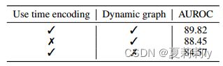
        ②Test of hidden size and layers:

2.5. Conclusion

        Their TENET provide valuable interpretability

3. Reference List

Kim B. et al. (2023) 'Large-scale Graph Representation Learning of Dynamic Brain Connectome with Transformers', NeurIPS. doi: https://doi.org/10.48550/arXiv.2312.14939