Pandas应用-股票分析实战

股票时间序列

时间序列：
金融领域最重要的数据类型之一
股价、汇率为常见的时间序列数据
趋势分析：
主要分析时间序列在某一方向上持续运动
在量化交易领域，我们通过统计手段对投资品的收益率进行时间序列建模，以此来预测未来的收益率并产生交易信
序列相关性：
金融时间序列的一个最重要特征是序列相关性
以投资品的收益率序列为例，我们会经常观察到一段时间内的收益率之间存在正相关或者负相关

Pandas时间序列函数

datetime：
时间序列最常用的数据类型
方便进行各种时间类型运算
loc：
Pandas中对DateFrame进行筛选的函数，相当于SQL中的where
groupby：
Pandas中对数据分组函数，相当于SQL中的GroupBy
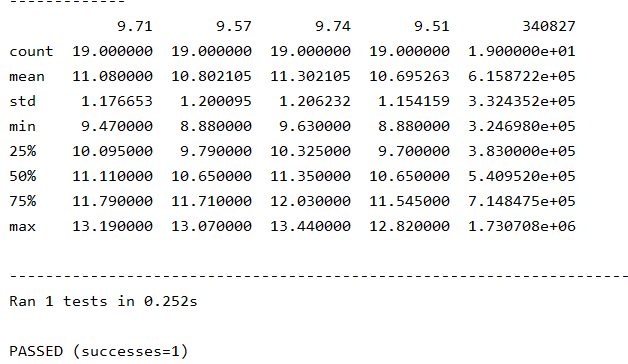
读取数据

    def testReadFile(self):
        file_name = r"D:\lhjytest\demo.csv"
        df = pd.read_csv(file_name)

        print(df.info())
        print("-------------")
        print(df.describe())

时间处理

    def testTime(self):
        file_name = r"D:\lhjytest\demo.csv"
        df = pd.read_csv(file_name)
        df.columns = ["stock_id","date","close","open","high","low","volume"]
        df["date"] = pd.to_datetime(df["date"])
        df["year"] = df["date"].dt.year
        df["month"] = df["date"].dt.month
        print(df)

最低收盘价

    def testCloseMin(self):
        file_name = r"D:\lhjytest\demo.csv"
        df = pd.read_csv(file_name)
        df.columns = ["stock_id","date","close","open","high","low","volume"]

        print("""close min : {}""".format(df["close"].min()))
        print("""close min index : {}""".format(df["close"].idxmin()))
        print("""close min frame : {}""".format(df.loc[df["close"].idxmin()]))

每月平均收盘价与开盘价

    def testMean(self):
        file_name = r"D:\lhjytest\demo.csv"
        df = pd.read_csv(file_name)
        df.columns = ["stock_id","date","close","open","high","low","volume"]

        df["date"] = pd.to_datetime(df["date"])
        df["month"] = df["date"].dt.month

        print("""month close mean : {}""".format(df.groupby("month")["close"].mean()))
        print("""month open mean : {}""".format(df.groupby("month")["open"].mean()))

算涨跌幅

# 涨跌幅今日收盘价减去昨日收盘价
    def testRipples_ratio(self):
        file_name = r"D:\lhjytest\demo.csv"
        df = pd.read_csv(file_name)
        df.columns = ["stock_id","date","close","open","high","low","volume"]

        df["date"] = pd.to_datetime(df["date"])

        df["rise"] = df["close"].diff()
        df["rise_ratio"] = df["rise"] / df.shift(-1)["close"]

        print(df)

计算股价移动平均

def testMA(self):
    file_name = r"D:\lhjytest\demo.csv"
    df = pd.read_csv(file_name)
    df.columns = ["stock_id","date","close","open","high","low","volume"]

    df['ma_5'] = df.close.rolling(window=5).mean()
    df['ma_10'] = df.close.rolling(window=10).mean()
    df = df.fillna(0)

    print(df)

K线图

K线图
K线图蕴含大量信息，能显示股价的强弱、多空双方的力量对比，是技术分析最常见的工具

K线图实现

Matplotlib
一个Python 的 2D绘图库,窗以各种硬拷贝格式和跨平台的交互式环境生成出版质量级别的图形
matplotlib finance
python 中可以用来画出蜡烛图线图的分析工具，目前已经从 matplotlib 中独立出来
读取股票数据，画出K线图

    def testKLineChart(self):
        file_name = r"D:\lhjytest\demo.csv"
        df = pd.read_csv(file_name)
        df.columns = ["stock_id","date","close","open","high","low","volume"]

        fig = plt.figure()
        axes = fig.add_subplot(111)
        candlestick2_ochl(ax=axes,opens=df["open"].values,closes=df["close"].values,highs=df["high"].values,
                          lows=df["low"].values,width=0.75,colorup='red',colordown='green')
        plt.xticks(range(len(df.index.values)),df.index.values,rotation=30)
        axes.grid(True)
        plt.title("K-Line")
        plt.show()

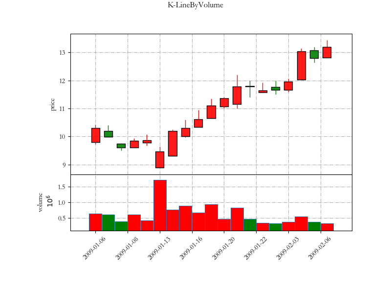
 def testKLineByVolume(self):
        file_name = r"D:\lhjytest\demo.csv"
        df = pd.read_csv(file_name)
        df.columns = ["stock_id","date","close","open","high","low","volume"]
        df = df[["date","close","open","high","low","volume"]]
        df["date"] = pd.to_datetime(df["date"])
        df = df.set_index('date')

        my_color = mpf.make_marketcolors(
            up = 'red',
            down = 'green',
            wick = 'i',
            volume = {'up':'red','down':'green'},
            ohlc = 'i'
        )

        my_style  = mpf.make_mpf_style(
            marketcolors = my_color,
            gridaxis = 'both',
            gridstyle = '-.',
            rc = {'font.family':'STSong'}
        )

        mpf.plot(
            df,
            type = 'candle',
            title = 'K-LineByVolume',
            ylabel = 'price',
            style = my_style,
            show_nontrading = False,
            volume = True,
            ylabel_lower = 'volume',
            datetime_format = '%Y-%m-%d',
            xrotation = 45,
            linecolor = '#00ff00',
            tight_layout = False
        )

K线图带交易量及均线

   def testKLineByMA(self):
        file_name = r"D:\lhjytest\demo.csv"
        df = pd.read_csv(file_name)
        df.columns = ["stock_id","date","close","open","high","low","volume"]
        df = df[["date","close","open","high","low","volume"]]
        df["date"] = pd.to_datetime(df["date"])
        df = df.set_index('date')

        my_color = mpf.make_marketcolors(
            up = 'red',
            down = 'green',
            wick = 'i',
            volume = {'up':'red','down':'green'},
            ohlc = 'i'
        )

        my_style  = mpf.make_mpf_style(
            marketcolors = my_color,
            gridaxis = 'both',
            gridstyle = '-.',
            rc = {'font.family':'STSong'}
        )

        mpf.plot(
            df,
            type = 'candle',
            mav = [5,10],
            title='K-LineByVolume',
            ylabel='price',
            style=my_style,
            show_nontrading=False,
            volume=True,
            ylabel_lower='volume',
            datetime_format='%Y-%m-%d',
            xrotation=45,
            linecolor='#00ff00',
            tight_layout=False
        )