Python 对海表面温度进行EOF分解与前n模态合成
一、EOF分解
- 数据来源:来自NOAA的2017-2021年0.25°×0.25°的日平均OISST数据(海表面温度数据)。
- 关于EOF的理解:利用2017-2020年4年数据进行EOF分解,2021年1月1日的数据来做合成检验。对长度是1461的二维海表面温度数据进行分解,分解得到的时间序列一共1461组长度1461的时间序列,一共1461个二维空间模态。按照方差大小从前到后。
- 代码实现:
import numpy as np
import pandas as pd
import matplotlib.pyplot as plt
from netCDF4 import Dataset
import datetime
from datetime import timedelta,datetime,date
from eofs.standard import Eof
import eofs
import cartopy.crs as ccrs
import cartopy.feature as cfeature
from cartopy.mpl.ticker import LongitudeFormatter,LatitudeFormatter
scale='10m'
proj=ccrs.PlateCarree(central_longitude=180)
tran=ccrs.PlateCarree()
df='obs025.nc'
f=Dataset(df)
lon=f.variables['lon'][:]
lat=f.variables['lat'][:]
ssto=f.variables['obssst'][:]
lat=lat[:640]
ssto=ssto[:-365,:640,:]
lon1=0
lon2=360
lat1=-90
lat2=70
num=4
lat=np.array(lat)
coslat=np.cos(np.deg2rad(lat))
wgts=np.sqrt(coslat)[...,np.newaxis] #权重
solver=Eof(ssto,weights=wgts) #eof分解
eof=solver.eofs(eofscaling=2) #空间模态 乘以特征值的平方根
pc=solver.pcs() #时间系数,默认pcscaling=0
var=solver.varianceFraction() #方差贡献
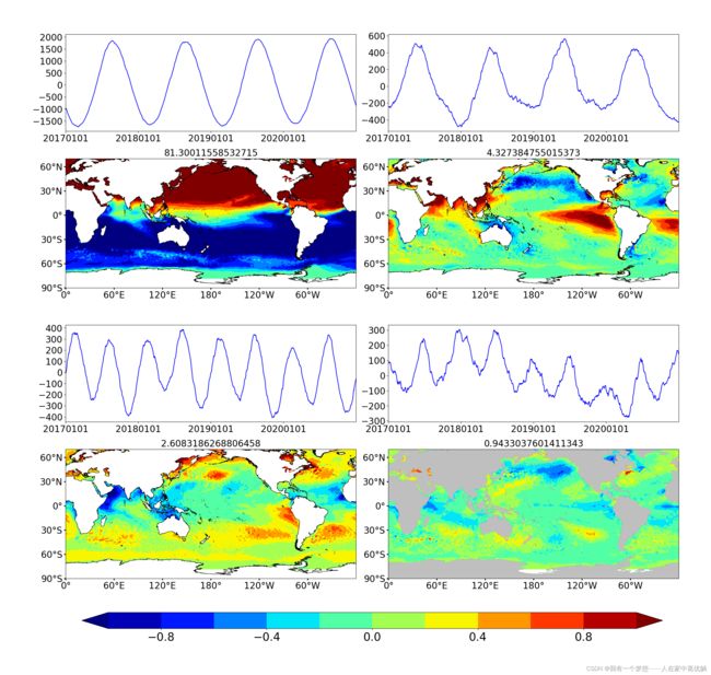
二、分解的序列与模态可视化。绘制前四个模态的模态与序列
代码如下:
time1=date(2017, 1, 1)
time2=date(2020,12,31)
t=pd.date_range(time1,time2,freq='D')
def eofall(name): #将模态和时间系数进行画图
fig=plt.figure(figsize=(20,20))
ax=fig.add_axes([0.025,0.78,0.45,0.15])
ax.plot(t,pc[:,0],c='b')
xticks=pd.date_range(time1,time2,freq='12MS')
ax.set_xticks(xticks)
ax.set_xticklabels(xticks.strftime('%Y%m%d'))
ax.set_xlim(min(t),max(t))
plt.xticks(fontsize=20)
plt.yticks(fontsize=20)
ax=fig.add_axes([0.525,0.78,0.45,0.15])
ax.plot(t,pc[:,1],c='b')
xticks=pd.date_range(time1,time2,freq='12MS')
ax.set_xticks(xticks)
ax.set_xticklabels(xticks.strftime('%Y%m%d'))
ax.set_xlim(min(t),max(t))
plt.xticks(fontsize=20)
plt.yticks(fontsize=20)
ax=fig.add_axes([0.025,0.28+0.05,0.45,0.15])
ax.plot(t,pc[:,2],c='b')
xticks=pd.date_range(time1,time2,freq='12MS')
ax.set_xticks(xticks)
ax.set_xticklabels(xticks.strftime('%Y%m%d'))
ax.set_xlim(min(t),max(t))
plt.xticks(fontsize=20)
plt.yticks(fontsize=20)
ax=fig.add_axes([0.525,0.28+0.05,0.45,0.15])
ax.plot(t,pc[:,3],c='b')
xticks=pd.date_range(time1,time2,freq='12MS')
ax.set_xticks(xticks)
ax.set_xticklabels(xticks.strftime('%Y%m%d'))
ax.set_xlim(min(t),max(t))
plt.xticks(fontsize=20)
plt.yticks(fontsize=20)
ax1=fig.add_axes([0.025,0.525,0.45,0.225],projection=ccrs.PlateCarree(
central_longitude=180))
ax1.add_feature(cfeature.COASTLINE.with_scale(scale),lw=0.75)
land=cfeature.NaturalEarthFeature('physical','land',scale,edgecolor='face',
facecolor=cfeature.COLORS['land'])
lon_formatter=LongitudeFormatter(zero_direction_label=False)
lat_formatter=LatitudeFormatter()
ax1.xaxis.set_major_formatter(lon_formatter)
ax1.yaxis.set_major_formatter(lat_formatter)
ax1.set_xticks(np.arange(lon1,lon2,60),crs=ccrs.PlateCarree())
ax1.set_yticks(np.arange(lat1,lat2,30),crs=ccrs.PlateCarree())
ax1.set_xlim(-180,180)
ax1.set_ylim(-90,70)
ax1.tick_params(width=2,colors='k')
plt.xticks(fontsize=20)
plt.yticks(fontsize=20)
plt.contourf(lon,lat,eof[0,:,:],transform=ccrs.PlateCarree(),cmap='jet',
levels=np.arange(-1,1.1,0.2),extend='both')
plt.title(var[0]*100,fontsize=20)
ax1=fig.add_axes([0.525,0.525,0.45,0.2255],projection=ccrs.PlateCarree(
central_longitude=180))
ax1.add_feature(cfeature.COASTLINE.with_scale(scale),lw=0.75)
land=cfeature.NaturalEarthFeature('physical','land',scale,edgecolor='face',
facecolor=cfeature.COLORS['land'])
lon_formatter=LongitudeFormatter(zero_direction_label=False)
lat_formatter=LatitudeFormatter()
ax1.xaxis.set_major_formatter(lon_formatter)
ax1.yaxis.set_major_formatter(lat_formatter)
ax1.set_xticks(np.arange(lon1,lon2,60),crs=ccrs.PlateCarree())
ax1.set_yticks(np.arange(lat1,lat2,30),crs=ccrs.PlateCarree())
ax1.set_xlim(-180,180)
ax1.set_ylim(-90,70)
ax1.tick_params(width=2,colors='k')
plt.xticks(fontsize=20)
plt.yticks(fontsize=20)
plt.contourf(lon,lat,eof[1,:,:],transform=ccrs.PlateCarree(),cmap='jet',
levels=np.arange(-1,1.1,0.2),extend='both')
plt.title(var[1]*100,fontsize=20)
ax1=fig.add_axes([0.025,0.025+0.05,0.45,0.225],projection=ccrs.PlateCarree(
central_longitude=180))
ax1.add_feature(cfeature.COASTLINE.with_scale(scale),lw=0.75)
land=cfeature.NaturalEarthFeature('physical','land',scale,edgecolor='face',
facecolor=cfeature.COLORS['land'])
lon_formatter=LongitudeFormatter(zero_direction_label=False)
lat_formatter=LatitudeFormatter()
ax1.xaxis.set_major_formatter(lon_formatter)
ax1.yaxis.set_major_formatter(lat_formatter)
ax1.set_xticks(np.arange(lon1,lon2,60),crs=ccrs.PlateCarree())
ax1.set_yticks(np.arange(lat1,lat2,30),crs=ccrs.PlateCarree())
ax1.set_xlim(-180,180)
ax1.set_ylim(-90,70)
ax1.tick_params(width=2,colors='k')
plt.xticks(fontsize=20)
plt.yticks(fontsize=20)
plt.contourf(lon,lat,eof[2,:,:],transform=ccrs.PlateCarree(),cmap='jet',
levels=np.arange(-1,1.1,0.2),extend='both')
plt.title(var[2]*100,fontsize=20)
ax1=fig.add_axes([0.525,0.025+0.05,0.45,0.225],projection=ccrs.PlateCarree(
central_longitude=180))
ax1.add_feature(cfeature.COASTLINE.with_scale(scale),lw=0.75)
land=cfeature.NaturalEarthFeature('physical','land',scale,edgecolor='face',
facecolor=cfeature.COLORS['land'])
ax1.add_feature(land,facecolor='0.75')
lon_formatter=LongitudeFormatter(zero_direction_label=False)
lat_formatter=LatitudeFormatter()
ax1.xaxis.set_major_formatter(lon_formatter)
ax1.yaxis.set_major_formatter(lat_formatter)
ax1.set_xticks(np.arange(lon1,lon2,60),crs=ccrs.PlateCarree())
ax1.set_yticks(np.arange(lat1,lat2,30),crs=ccrs.PlateCarree())
ax1.set_xlim(-180,180)
ax1.set_ylim(-90,70)
ax1.tick_params(width=2,colors='k')
plt.xticks(fontsize=20)
plt.yticks(fontsize=20)
plt.contourf(lon,lat,eof[3,:,:],transform=ccrs.PlateCarree(),cmap='jet',
levels=np.arange(-1,1.1,0.2),extend='both')
plt.title(var[3]*100,fontsize=20)
cb=plt.colorbar(cax=fig.add_axes([0.05,0.01,0.9,0.025]),orientation='horizontal')
cb.ax.tick_params(labelsize=25)
plt.savefig(name,bbox_inches='tight',pad_inches=1)
eofall('eof2017-2020.png')
结果展示:
三、前4个模态合成SST并比较合成SST与真实SST的差异
代码:
df='obs025.nc'
f=Dataset(df)
lon=f.variables['lon'][:]
lat=f.variables['lat'][:]
ssto=f.variables['obssst'][:]
lat=lat[:640]
ssto=ssto[:-365,:640,:]
lon1=0
lon2=360
lat1=-90
lat2=70
num=4
lat=np.array(lat)
coslat=np.cos(np.deg2rad(lat))
wgts=np.sqrt(coslat)[...,np.newaxis] #权重
solver=Eof(ssto,weights=wgts) #eof分解
eof=solver.eofs() #空间模态
pc=solver.pcs() #时间系数,默认pcscaling=0
var=solver.varianceFraction() #方差贡献
与开始的eof分解略有不同,在进行分解及可视化的时候,将eof分解得到的空间模态乘以特征值的平方根来更好的展示效果。
def drawphotos(data1,data2,data3,name):
fig=plt.figure(figsize=(10,15))
for i in range(1,4):
ax=plt.subplot(3,1,i,projection=proj)
ax.add_feature(cfeature.COASTLINE.with_scale(scale),lw=0.75)
lon_formatter=LongitudeFormatter(zero_direction_label=False)
lat_formatter=LatitudeFormatter()
ax.xaxis.set_major_formatter(lon_formatter)
ax.yaxis.set_major_formatter(lat_formatter)
ax.set_xticks(np.arange(lon1,lon2,60),crs=tran)
ax.set_yticks(np.arange(lat1,lat2,30),crs=tran)
ax.set_xlim(-180,180)
ax.set_ylim(-90,70)
if i==3:
img=ax.contourf(lon,lat,data3,transform=tran,cmap='bwr',
levels=np.arange(-2,2.1,0.2),extend='both')
if i==1:
img=ax.contourf(lon,lat,data1,transform=tran,cmap='jet',
levels=np.arange(-4,32,2),extend='both')
if i==2:
img=ax.contourf(lon,lat,data2,transform=tran,cmap='jet',
levels=np.arange(-4,32,2),extend='both')
cb=plt.colorbar(img)
cb.ax.tick_params(labelsize=15)
plt.xticks(fontsize=15)
plt.yticks(fontsize=15)
plt.savefig(name,bbox_inches='tight',pad_inches=0)
sstobs1=np.zeros((len(lat),len(lon)))
for i in range(4):
print(pc[-365,i])
sstobs1=pc[-365,i]*eof[i,:,:]+sstobs1
sstobs1=sstobs1/np.broadcast_arrays(ssto,wgts)[1][0]
sstobs=sstobs1+np.mean(ssto,0)
bias=sstobs-ssto[-365,:,:]
drawphotos(ssto[-365,:,:],sstobs,bias,'obssstandbias4.png')
结果展示:
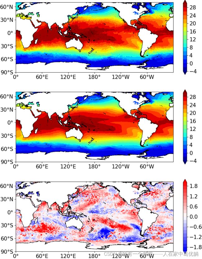 从上到下分别是2021年1月1日真实SST空间分布、前四个模态合成SST空间分布、两者之差。