深度学习革命背后:DBN、AlexNet、GAN 等神级架构,究竟藏着怎样的 AI 崛起密码?(附deepseek)
深度学习革命
-
-
- **3. 深度学习革命(2006年至今)**
-
- **2006年:深度学习奠基——深度信念网络(DBN)**
- **2012年:AlexNet崛起**
- **2014年:架构创新潮**
-
- **生成对抗网络(GAN)**
- **残差网络(ResNet)**
- **Transformer**
- **总结**
- 补充(deepseek)
-
- 一、核心技术原理
-
- 1. **混合专家架构(MoE)**
- 2. **多头潜在注意力(MLA)**
- 3. **多Token预测(MTP)**
- 4. **强化学习框架(GRPO)**
- 二、关键公式推导
-
- 1. **MoE门控计算**
- 2. **MLA注意力计算**
- 3. **GRPO优势函数**
- 三、代码实现要点
-
- 1. **MoE模块实现(PyTorch示例)**
- 2. **MTP损失实现**
- 3. **GRPO策略优化核心**
- 四、性能优化策略
-
3. 深度学习革命(2006年至今)
2006年:深度学习奠基——深度信念网络(DBN)
数学原理
DBN由多层受限玻尔兹曼机(RBM)堆叠而成,通过无监督预训练初始化权重,再通过反向传播微调。
- RBM的能量函数:
E ( v , h ) = − ∑ i a i v i − ∑ j b j h j − ∑ i , j v i w i j h j E(v, h) = -\sum_{i} a_i v_i - \sum_{j} b_j h_j - \sum_{i,j} v_i w_{ij} h_j E(v,h)=−i∑aivi−j∑bjhj−i,j∑viwijhj
其中 ( v ) 是可见层,( h ) 是隐藏层,( a )、( b ) 是偏置,( w_{ij} ) 是权重。 - 联合概率分布:
P ( v , h ) = 1 Z e − E ( v , h ) ( Z 为 归 一 化 因 子 ) P(v, h) = \frac{1}{Z} e^{-E(v, h)} \quad (Z为归一化因子) P(v,h)=Z1e−E(v,h)(Z为归一化因子) - 对比散度(CD-k)训练:
通过采样更新权重:
Δ w i j = η ( ⟨ v i h j ⟩ data − ⟨ v i h j ⟩ recon ) \Delta w_{ij} = \eta (\langle v_i h_j \rangle_{\text{data}} - \langle v_i h_j \rangle_{\text{recon}}) Δwij=η(⟨vihj⟩data−⟨vihj⟩recon)
代码实现(RBM训练)
import numpy as np

class RBM:
    def __init__(self, n_visible, n_hidden):
        self.W = np.random.randn(n_visible, n_hidden) * 0.1
        self.a = np.zeros(n_visible)
        self.b = np.zeros(n_hidden)

    def sigmoid(self, x):
        return 1 / (1 + np.exp(-x))

    def sample_h(self, v):
        h_prob = self.sigmoid(np.dot(v, self.W) + self.b)
        return h_prob, np.random.binomial(1, h_prob)

    def sample_v(self, h):
        v_prob = self.sigmoid(np.dot(h, self.W.T) + self.a)
        return v_prob, np.random.binomial(1, v_prob)

    def train(self, data, lr=0.01, k=1, epochs=100):
        for _ in range(epochs):
            for v0 in data:
                # Positive phase
                h0_prob, h0 = self.sample_h(v0)
                # Negative phase (CD-k)
                vk = v0
                for _ in range(k):
                    _, hk = self.sample_h(vk)
                    vk_prob, vk = self.sample_v(hk)
                # Update weights
                self.W += lr * (np.outer(v0, h0_prob) - np.outer(vk, hk))
                self.a += lr * (v0 - vk_prob)
                self.b += lr * (h0_prob - hk)

# 示例:训练RBM学习MNIST数据
from sklearn.datasets import fetch_openml
mnist = fetch_openml('mnist_784', version=1)
data = mnist.data / 255.0
data = np.round(data)  # 二值化

rbm = RBM(n_visible=784, n_hidden=256)
rbm.train(data.sample(1000), epochs=10)
论文链接
Hinton, G. E., et al. (2006). A Fast Learning Algorithm for Deep Belief Nets. Neural Computation.
2012年:AlexNet崛起
架构创新
- ReLU激活函数:解决梯度消失,加速训练。
ReLU ( x ) = max ( 0 , x ) \text{ReLU}(x) = \max(0, x) ReLU(x)=max(0,x) - Dropout层:随机屏蔽神经元防止过拟合(训练时以概率 ( p ) 关闭节点)。
- 多GPU并行:首次利用GPU加速训练。
AlexNet架构(简化版)
import torch
import torch.nn as nn

class AlexNet(nn.Module):
    def __init__(self, num_classes=1000):
        super().__init__()
        self.features = nn.Sequential(
            nn.Conv2d(3, 96, kernel_size=11, stride=4),  # 输入224x224x3 → 55x55x96
            nn.ReLU(inplace=True),
            nn.MaxPool2d(kernel_size=3, stride=2),       # → 27x27x96
            nn.Conv2d(96, 256, kernel_size=5, padding=2), # → 27x27x256
            nn.ReLU(inplace=True),
            nn.MaxPool2d(kernel_size=3, stride=2),        # → 13x13x256
            nn.Conv2d(256, 384, kernel_size=3, padding=1),# → 13x13x384
            nn.ReLU(inplace=True),
            nn.Conv2d(384, 384, kernel_size=3, padding=1),# → 13x13x384
            nn.ReLU(inplace=True),
            nn.Conv2d(384, 256, kernel_size=3, padding=1),# → 13x13x256
            nn.ReLU(inplace=True),
            nn.MaxPool2d(kernel_size=3, stride=2),        # → 6x6x256
        )
        self.classifier = nn.Sequential(
            nn.Dropout(),
            nn.Linear(256*6*6, 4096),
            nn.ReLU(inplace=True),
            nn.Dropout(),
            nn.Linear(4096, 4096),
            nn.ReLU(inplace=True),
            nn.Linear(4096, num_classes),
        )

    def forward(self, x):
        x = self.features(x)
        x = x.view(x.size(0), 256*6*6)
        x = self.classifier(x)
        return x

# 示例:在CIFAR-10上训练简化版AlexNet
model = AlexNet(num_classes=10)
criterion = nn.CrossEntropyLoss()
optimizer = torch.optim.SGD(model.parameters(), lr=0.01, momentum=0.9)
论文链接
Krizhevsky, A., et al. (2012). ImageNet Classification with Deep Convolutional Neural Networks. NeurIPS.
2014年:架构创新潮
生成对抗网络(GAN)
数学原理
- 目标函数(最小最大博弈):
min G max D V ( D , G ) = E x ∼ p data [ log D ( x ) ] + E z ∼ p z [ log ( 1 − D ( G ( z ) ) ) ] \min_G \max_D V(D, G) = \mathbb{E}_{x \sim p_{\text{data}}}[\log D(x)] + \mathbb{E}_{z \sim p_z}[\log(1 - D(G(z)))] GminDmaxV(D,G)=Ex∼pdata[logD(x)]+Ez∼pz[log(1−D(G(z)))] - 生成器 ( G ) 生成假数据,判别器 ( D ) 区分真假。
代码实现(MNIST生成)
import torch
import torch.nn as nn

class Generator(nn.Module):
    def __init__(self):
        super().__init__()
        self.model = nn.Sequential(
            nn.Linear(100, 256),
            nn.LeakyReLU(0.2),
            nn.Linear(256, 512),
            nn.LeakyReLU(0.2),
            nn.Linear(512, 784),
            nn.Tanh()
        )

    def forward(self, z):
        return self.model(z)

class Discriminator(nn.Module):
    def __init__(self):
        super().__init__()
        self.model = nn.Sequential(
            nn.Linear(784, 512),
            nn.LeakyReLU(0.2),
            nn.Linear(512, 256),
            nn.LeakyReLU(0.2),
            nn.Linear(256, 1),
            nn.Sigmoid()
        )

    def forward(self, x):
        return self.model(x)

# 训练循环
G = Generator()
D = Discriminator()
opt_G = torch.optim.Adam(G.parameters(), lr=0.0002)
opt_D = torch.optim.Adam(D.parameters(), lr=0.0002)

for epoch in range(100):
    for real_images, _ in dataloader:
        # 训练判别器
        z = torch.randn(batch_size, 100)
        fake_images = G(z)
        real_loss = torch.log(D(real_images)).mean()
        fake_loss = torch.log(1 - D(fake_images.detach())).mean()
        loss_D = -(real_loss + fake_loss)
        opt_D.zero_grad()
        loss_D.backward()
        opt_D.step()

        # 训练生成器
        loss_G = -torch.log(D(fake_images)).mean()
        opt_G.zero_grad()
        loss_G.backward()
        opt_G.step()
论文链接
Goodfellow, I., et al. (2014). Generative Adversarial Nets. NeurIPS.
残差网络(ResNet)
数学原理
残差块通过跳跃连接传递梯度:
y = F ( x , { W i } ) + x y = F(x, \{W_i\}) + x y=F(x,{Wi})+x
其中 ( F ) 是残差函数(如两个卷积层),( x ) 是输入。
代码实现(ResNet-18)
class ResidualBlock(nn.Module):
    def __init__(self, in_channels, out_channels, stride=1):
        super().__init__()
        self.conv1 = nn.Conv2d(in_channels, out_channels, kernel_size=3, stride=stride, padding=1)
        self.bn1 = nn.BatchNorm2d(out_channels)
        self.conv2 = nn.Conv2d(out_channels, out_channels, kernel_size=3, padding=1)
        self.bn2 = nn.BatchNorm2d(out_channels)
        self.shortcut = nn.Sequential()
        if stride != 1 or in_channels != out_channels:
            self.shortcut = nn.Sequential(
                nn.Conv2d(in_channels, out_channels, kernel_size=1, stride=stride),
                nn.BatchNorm2d(out_channels)
            )

    def forward(self, x):
        out = F.relu(self.bn1(self.conv1(x)))
        out = self.bn2(self.conv2(out))
        out += self.shortcut(x)
        out = F.relu(out)
        return out

class ResNet18(nn.Module):
    def __init__(self, num_classes=10):
        super().__init__()
        self.conv1 = nn.Conv2d(3, 64, kernel_size=7, stride=2, padding=3)
        self.bn1 = nn.BatchNorm2d(64)
        self.maxpool = nn.MaxPool2d(kernel_size=3, stride=2, padding=1)
        self.layer1 = self._make_layer(64, 64, 2, stride=1)
        self.layer2 = self._make_layer(64, 128, 2, stride=2)
        self.layer3 = self._make_layer(128, 256, 2, stride=2)
        self.layer4 = self._make_layer(256, 512, 2, stride=2)
        self.avgpool = nn.AdaptiveAvgPool2d((1,1))
        self.fc = nn.Linear(512, num_classes)

    def _make_layer(self, in_channels, out_channels, blocks, stride):
        layers = [ResidualBlock(in_channels, out_channels, stride)]
        for _ in range(1, blocks):
            layers.append(ResidualBlock(out_channels, out_channels))
        return nn.Sequential(*layers)

    def forward(self, x):
        x = F.relu(self.bn1(self.conv1(x)))
        x = self.maxpool(x)
        x = self.layer1(x)
        x = self.layer2(x)
        x = self.layer3(x)
        x = self.layer4(x)
        x = self.avgpool(x)
        x = x.view(x.size(0), -1)
        x = self.fc(x)
        return x
论文链接
He, K., et al. (2016). Deep Residual Learning for Image Recognition. CVPR.
Transformer
数学原理
- 自注意力机制:
Attention ( Q , K , V ) = softmax ( Q K T d k ) V \text{Attention}(Q, K, V) = \text{softmax}\left( \frac{QK^T}{\sqrt{d_k}} \right) V Attention(Q,K,V)=softmax(dkQKT)V - 位置编码(正弦函数):
P E ( p o s , 2 i ) = sin ( p o s / 1000 0 2 i / d ) PE_{(pos, 2i)} = \sin\left(pos / 10000^{2i/d}\right) PE(pos,2i)=sin(pos/100002i/d)
P E ( p o s , 2 i + 1 ) = cos ( p o s / 1000 0 2 i / d ) PE_{(pos, 2i+1)} = \cos\left(pos / 10000^{2i/d}\right) PE(pos,2i+1)=cos(pos/100002i/d)
代码实现(Transformer编码器层)
class TransformerEncoderLayer(nn.Module):
    def __init__(self, d_model, nhead, dim_feedforward=2048, dropout=0.1):
        super().__init__()
        self.self_attn = nn.MultiheadAttention(d_model, nhead, dropout=dropout)
        self.linear1 = nn.Linear(d_model, dim_feedforward)
        self.dropout = nn.Dropout(dropout)
        self.linear2 = nn.Linear(dim_feedforward, d_model)
        self.norm1 = nn.LayerNorm(d_model)
        self.norm2 = nn.LayerNorm(d_model)
        self.activation = nn.ReLU()

    def forward(self, src, src_mask=None):
        # 自注意力
        src2 = self.self_attn(src, src, src, attn_mask=src_mask)[0]
        src = src + self.dropout(src2)
        src = self.norm1(src)
        # 前馈网络
        src2 = self.linear2(self.dropout(self.activation(self.linear1(src))))
        src = src + self.dropout(src2)
        src = self.norm2(src)
        return src

# 示例:编码句子
encoder_layer = TransformerEncoderLayer(d_model=512, nhead=8)
src = torch.rand(10, 32, 512)  # (序列长度, 批大小, 特征维度)
out = encoder_layer(src)
论文链接
Vaswani, A., et al. (2017). Attention Is All You Need. NeurIPS.
总结
- DBN:通过无监督预训练解锁深层网络潜力。
- AlexNet:GPU与大数据推动CNN成为视觉任务霸主。
- GAN:生成模型进入对抗时代。
- ResNet:残差连接突破网络深度极限。
- Transformer:自注意力机制颠覆序列建模范式。
这些创新构成深度学习的核心骨架,驱动AI从实验室走向工业级应用。
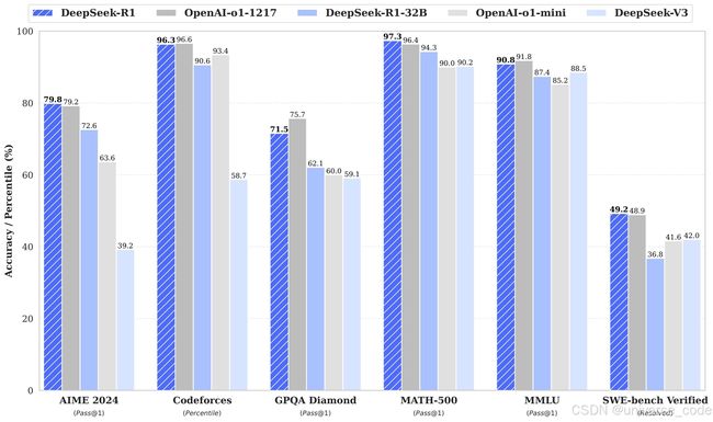
补充(deepseek)
一、核心技术原理
1. 混合专家架构(MoE)
采用 动态参数激活机制,总参数量达671B的DeepSeek-V3模型中,每个token仅激活37B参数。其核心实现为:
- 门控网络:通过稀疏门控函数动态选择专家
- 负载均衡策略:采用无辅助损失负载均衡算法,确保专家激活频率均衡
2. 多头潜在注意力(MLA)
改进传统注意力机制,在128K上下文窗口下显存占用减少50%。核心创新:
- 潜在注意力头:通过动态选择机制激活不同注意力头
- 稀疏计算优化:对长距离依赖采用稀疏矩阵计算
3. 多Token预测(MTP)
同时预测未来N个token(N=4),训练效率提升3.2倍。损失函数设计为:
L M T P = ∑ i = 1 N λ i ⋅ CrossEntropy ( y t + i , y ^ t + i ) \mathcal{L}_{MTP} = \sum_{i=1}^N \lambda_i \cdot \text{CrossEntropy}(y_{t+i}, \hat{y}_{t+i}) LMTP=i=1∑Nλi⋅CrossEntropy(yt+i,y^t+i)
其中 λ i \lambda_i λi为衰减系数(如0.9^i)
4. 强化学习框架(GRPO)
群体相对策略优化框架的核心公式:
E ( s , a ) ∼ π [ π ( a ∣ s ) π o l d ( a ∣ s ) A ^ ( s , a ) − β ⋅ KL ( π ∣ ∣ π o l d ) ] \mathbb{E}_{(s,a)\sim\pi} \left[ \frac{\pi(a|s)}{\pi_{old}(a|s)} \hat{A}(s,a) - \beta \cdot \text{KL}(\pi||\pi_{old}) \right] E(s,a)∼π[πold(a∣s)π(a∣s)A^(s,a)−β⋅KL(π∣∣πold)]
其中 A ^ ( s , a ) \hat{A}(s,a) A^(s,a)为相对优势函数,通过群体策略比较计算。
二、关键公式推导
1. MoE门控计算
门控分数计算式:
g ( x ) = Softmax ( W g ⋅ x + ϵ ) g(x) = \text{Softmax}(W_g \cdot x + \epsilon) g(x)=Softmax(Wg⋅x+ϵ)
其中 ϵ ∼ N ( 0 , σ 2 ) \epsilon \sim \mathcal{N}(0, \sigma^2) ϵ∼N(0,σ2)为噪声注入, W g ∈ R d × E W_g \in \mathbb{R}^{d \times E} Wg∈Rd×E为门控权重矩阵。
2. MLA注意力计算
潜在注意力头选择:
h l a t e n t = arg max k ( MLP ( x ) ⋅ W h ) h_{latent} = \arg\max_k (\text{MLP}(x) \cdot W_h) hlatent=argkmax(MLP(x)⋅Wh)
实际计算仅激活top-K个注意力头。
3. GRPO优势函数
相对优势计算:
A ^ ( s , a ) = R ( s , a ) − μ R σ R \hat{A}(s,a) = \frac{R(s,a) - \mu_R}{\sigma_R} A^(s,a)=σRR(s,a)−μR
其中 μ R \mu_R μR和 σ R \sigma_R σR为当前策略群体中奖励的均值和标准差。
三、代码实现要点
1. MoE模块实现(PyTorch示例)
class MoE(nn.Module):
    def __init__(self, num_experts=8, capacity_factor=1.0):
        super().__init__()
        self.experts = nn.ModuleList([Expert() for _ in range(num_experts)])
        self.gate = nn.Linear(d_model, num_experts)
        self.cap_factor = capacity_factor

    def forward(self, x):
        gates = self.gate(x) # [B, T, E]
        indices = torch.topk(gates, k=2, dim=-1).indices # top-2路由
        expert_outputs = []
        for expert_idx in range(self.num_experts):
            mask = (indices == expert_idx)
            if mask.sum() > 0:
                expert_out = self.experts[expert_idx](x[mask])
                expert_outputs.append((expert_out, mask))
        return combine_outputs(expert_outputs) # 加权合并
2. MTP损失实现
class MTPloss(nn.Module):
    def __init__(self, n_predict=4):
        super().__init__()
        self.n = n_predict
        self.weights = [0.9**i for i in range(n)]

    def forward(self, logits, targets):
        total_loss = 0
        for i in range(self.n):
            shifted_logits = logits[:, :-i-1]
            shifted_targets = targets[:, i+1:]
            loss = F.cross_entropy(shifted_logits, shifted_targets)
            total_loss += self.weights[i] * loss
        return total_loss
3. GRPO策略优化核心
def grpo_update(policy, batch, beta=0.1):
    # 计算相对优势
    rewards = compute_rewards(batch)
    adv = (rewards - rewards.mean()) / (rewards.std() + 1e-8)

    # 策略梯度计算
    log_probs = policy.log_prob(batch.actions)
    ratios = torch.exp(log_probs - batch.old_log_probs)
    surr1 = ratios * adv
    surr2 = torch.clamp(ratios, 1-beta, 1+beta) * adv
    loss = -torch.min(surr1, surr2).mean()

    # KL散度约束
    kl = compute_kl_divergence(policy, batch)
    loss += kl_penalty * kl.mean()
    return loss
四、性能优化策略
- 分布式训练:采用3D并行(数据+模型+流水线),支持千卡级集群训练
- 量化推理:使用FP8混合精度训练,推理速度提升2.3倍
- 稀疏计算:对注意力矩阵应用Block-Sparse计算,显存占用降低40%
完整实现可参考官方代码及GRPO专项实现,如需特定组件的完整代码示例,可说明具体模块需求。