Q-Learning算法：从原理到路径搜索代码实现

一、引言

在人工智能和机器学习领域，强化学习是一种让智能体通过与环境交互，不断尝试和学习，以最大化累积奖励的学习范式。Q-Learning作为强化学习中的经典算法，以其简单高效的特点，在诸多领域得到了广泛应用，如机器人导航、游戏策略制定等。本文将详细介绍Q-Learning算法的原理，通过数学推导深入理解其核心思想，并结合一个路径搜索的Python代码示例，展示如何将Q-Learning算法应用到实际问题中。

二、强化学习基础

强化学习是一种机器学习范式，智能体通过与环境交互学习最优策略。其核心要素包括：

• 状态（State）：智能体所处环境的特征描述。
• 动作（Action）：智能体为改变状态而采取的操作。
• 奖励（Reward）：环境对智能体动作的一种评价信号。
• 策略（Policy）：智能体选择动作的规则，即给定状态下，采取各动作的概率分布。

三、Q-Learning算法

3.1 Q-Learning算法概述

Q-Learning是一种基于值函数的强化学习算法，旨在学习最优策略。其核心是学习一个Q值表（Q-table），用于评估在给定状态下采取某个动作的期望回报。

3.2 Q值的定义

Q值（状态-动作值函数）表示在状态 s 下执行动作 a 后，智能体的期望累积奖励。数学上定义为：
$$Q(s,a)=E_{\pi }[R_t+\gamma R_{t+1}+{\gamma }^2{R}_{t+2}+\cdots +{\gamma }^{n-1}{R}_{t+n}\mid S_t=s,A_t=a]$$
其中：

• $R_t$ 是执行动作后的奖励。
• $\gamma$ 是折扣因子（$0\le \gamma <1$），用于平衡短期和长期回报。

3.3 Q-Learning算法步骤

1. 初始化Q表：初始时，所有状态-动作对的Q值设为0或随机值。
2. 探索与利用：智能体通过$ϵ$-贪心策略选择动作：
   • 以概率$ϵ$随机选择动作（探索）。
   • 以概率$1-ϵ$选择当前Q值最高的动作（利用）。
3. 状态转移与奖励：执行动作，观察下一个状态和奖励。
4. Q值更新：根据以下公式更新Q值：

$$Q(s,a)\leftarrow Q(s,a)+\alpha [R+\gamma {max}_{a^{\prime }}Q(s^{\prime },a^{\prime })-Q(s,a)]$$

其中：

• $\alpha$是学习率（$0<\alpha \le 1$）。
• $R$ 是当前动作的奖励。
• ${max}_{a^{\prime }}Q(s^{\prime },a^{\prime })$ 表示下一个状态下的最大Q值。

3.4 Q-Learning的收敛（Bellman期望方程）

当智能体经历足够多的状态转移和动作选择后，Q值会逐渐收敛到最优值。根据Bellman期望方程，最优Q值满足：

$$Q^{\ast }(s,a)=E[R+\gamma {max}_{a^{\prime }}Q(s^{\prime },a^{\prime })]$$

四、参数的影响和选取建议

4.1 折扣率（Discount Factor）

• 影响：
  • 折扣率（通常用符号$\gamma$表示）衡量了未来奖励的重要性。折扣率的取值范围通常在0到1之间（不包括1）。如果折扣率接近于1，智能体会更加重视未来的奖励，有助于长期策略的优化；如果折扣率接近于0，智能体更加关注即时奖励，更注重短期回报。
  • 较高的折扣率意味着智能体愿意为了获得更大的长期回报而牺牲一些即时奖励，这有助于学习到更具前瞻性的策略。然而，过高的折扣率可能导致智能体过于关注未来的奖励，而忽视了当前的奖励，从而导致学习过程变得缓慢，甚至难以收敛。
• 选取建议：
  • 一般来说，折扣率的取值应该根据具体问题的性质和目标来确定。对于那些需要考虑长期回报的问题，可以设置较高的折扣率（如0.9或更高），以促使智能体学习到更优的长期策略。
  • 如果问题更注重短期回报，或者未来的奖励具有较大的不确定性，可以适当降低折扣率（如0.5或更低），使智能体更关注即时奖励。
  • 在实际应用中，可以通过实验和调试来确定最佳的折扣率。可以尝试不同的折扣率值，观察算法的收敛速度和最终性能，选择一个能够平衡短期和长期回报的折扣率。

4.2 学习率（Learning Rate）

• 影响：
  • 学习率（通常用符号$\alpha$表示）控制了Q值更新的速度。学习率决定了每次更新Q值时所采用的步长大小。如果学习率过大，可能导致Q值不断波动，无法收敛到最优解；如果学习率过小，可能导致算法收敛速度过慢。
  • 较高的学习率可以使智能体更快地学习到新的信息，但也可能导致Q值的波动较大，难以稳定下来。较低的学习率则可以使Q值更新更加平稳，但学习速度会变慢。
• 选取建议：
  • 一般建议初始时选择一个较大的学习率（如0.1或0.2），以加快算法的收敛速度。随着训练的进行，可以逐渐减小学习率，以避免Q值的震荡。
  • 可以采用学习率衰减的方法，即随着训练的进行，按照一定的规则逐渐减小学习率。
  • 在实际应用中，可以通过实验和调试来确定最佳的学习率。可以尝试不同的学习率值，观察算法的收敛速度和最终性能，选择一个能够使算法快速收敛且稳定的值。

4.3 探索率（Exploration Rate）

• 影响：
  • 探索率（通常用符号$ϵ$表示）用来平衡探索和利用的权衡。探索率决定了智能体在选择动作时进行随机探索的概率。如果探索率过高，智能体将倾向于尝试新的行为，可能导致无法充分利用已有的知识；如果探索率过低，智能体将倾向于选择已知的最优行为，可能导致陷入局部最优解。
• 选取建议：
  • 通常情况下，初始时可以选择一个较高的探索率（如0.1或0.2），以促使智能体充分探索环境。随着训练的进行，可以逐渐减小探索率，以增加利用已知知识的比例。
  • 可以采用$ϵ$-贪心策略的变体，如 ϵ-衰减策略，即随着训练的进行，按照一定的规则逐渐减小 ϵ 值。
  • 在实际应用中，可以通过实验和调试来确定最佳的探索率。可以尝试不同的探索率值，观察算法的收敛速度和最终性能，选择一个能够平衡探索和利用的值。

五、迷宫探索问题及代码实现

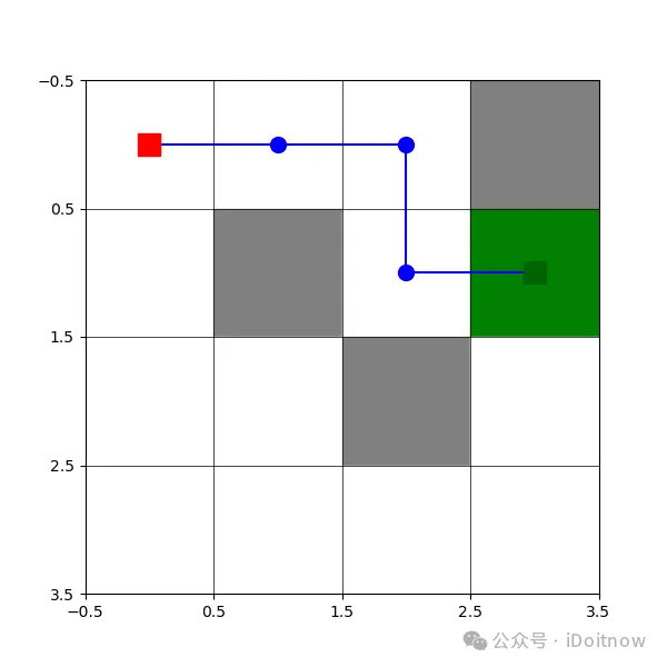
5.1 问题描述

我们要解决的问题是让一个智能体在一个迷宫中找到从起点到终点的最优路径。迷宫用一个二维数组表示，其中 S 表示起点，G 表示终点，. 表示可通行的路径，X 表示障碍物。智能体可以执行四个动作：向上、向下、向左、向右。

5.2 代码实现

import random
import matplotlib.pyplot as plt
import numpy as np

# 迷宫配置
maze = [
    ["S", ".", ".", "X"],
    [".", "X", ".", "G"],
    [".", ".", "X", "."],
    [".", ".", ".", "."]
]
rows, cols = len(maze), len(maze[0])
actions = ["up", "down", "left", "right"]

# 初始化可视化
plt.ion()
fig = plt.figure(figsize=(12, 10))
ax1 = plt.subplot2grid((2, 2), (0, 0))  # 迷宫可视化
ax2 = plt.subplot2grid((2, 2), (0, 1))  # Q值热力图
ax3 = plt.subplot2grid((2, 2), (1, 0), colspan=2)  # 学习曲线

# 新增GIF保存相关配置
from PIL import Image

gif_frames = []  # 用于存储动画帧
gif_path = "./maze_learning.gif"  # GIF保存路径


# 设置各子图初始参数
def init_plots():
    # 迷宫可视化设置
    ax1.set_title("Maze Exploration Process")
    ax1.set_aspect('equal')
    ax1.invert_yaxis()
    ax1.set_xlim(-0.5, cols - 0.5)
    ax1.set_ylim(rows - 0.5, -0.5)

    # Q值热力图设置
    ax2.set_title("Q-Value Heatmap")
    ax2.set_aspect('equal')

    # 学习曲线设置
    ax3.set_title("Reward Convergence Curve")
    ax3.set_xlabel('Training Epochs')
    ax3.set_ylabel('Accumulated Rewards')

episode_rewards = []

# 映射状态到索引
state_to_idx = {(r, c): i for i, (r, c) in enumerate([(r, c) for r in range(rows) for c in range(cols)])}
idx_to_state = {v: k for k, v in state_to_idx.items()}

# 判断动作是否有效
def is_valid_move(state, action):
    r, c = state
    if action == "up": r -= 1
    elif action == "down": r += 1
    elif action == "left": c -= 1
    elif action == "right": c += 1
    if r < 0 or r >= rows or c < 0 or c >= cols or maze[r][c] == "X":
        return False
    return True

# 获取下一个状态
def next_state(state, action):
    if not is_valid_move(state, action):
        return state  # 无效动作保持原地
    r, c = state
    if action == "up": r -= 1
    elif action == "down": r += 1
    elif action == "left": c -= 1
    elif action == "right": c += 1
    return (r, c)

# 奖励函数
def get_reward(state):
    r, c = state
    if maze[r][c] == "G": return 10  # 到达目标
    elif maze[r][c] == "X": return -10  # 撞到障碍
    else: return -1  # 每步的代价

# 初始化 Q 表
Q = np.zeros((len(state_to_idx), len(actions)))

# Q-Learning 参数
# 优化后的Q-Learning参数（增加衰减率和动量项）
alpha = 0.2  # 初始学习率（提高初始值加速学习）
gamma = 0.9  # 折扣因子（提高长期回报考虑）
epsilon = 1.0  # 初始探索率（实现衰减策略）
min_epsilon = 0.001  # 最小探索率
epsilon_decay = 0.9  # 探索率衰减系数
episodes = 100  # 增加训练轮次

# Q-Learning 主循环
for episode in range(episodes):
    # 动态参数衰减（优化学习扰动）
    epsilon = max(min_epsilon, epsilon * epsilon_decay)  # 指数衰减探索率
    alpha = max(0.01, alpha * 0.9)  # 学习率衰减
    
    state = (0, 0)
    total_reward = 0
    step_count = 0  # 记录每轮步数
    
    # 在Q-Learning主循环内部补充帧捕获
    while maze[state[0]][state[1]] != "G":
        # ε-贪心策略（增加基于步数的探索概率）
        if random.uniform(0, 1) < epsilon + (step_count/100):
            action_idx = random.randint(0, len(actions)-1)
        else:
            action_idx = np.argmax(Q[state_to_idx[state]])
        
        action = actions[action_idx]
        # 执行动作前获取当前状态索引
        state_idx = state_to_idx[state]  # 新增这行
        next_state_ = next_state(state, action)
        next_state_idx = state_to_idx[next_state_]
        reward = get_reward(next_state_)
        
        # 更新 Q 表
        Q[state_idx, action_idx] += alpha * (reward + gamma * np.max(Q[next_state_idx]) - Q[state_idx, action_idx])
        state = next_state_

        # 实时可视化
        ax1.clear()
        # 设置坐标轴
        ax1.set_title(f"Maze Exploration Process: {episode + 1}/{episodes}")
        ax1.set_aspect('equal')
        ax1.invert_yaxis()
        ax1.set_xlim(-0.5, cols - 0.5)
        ax1.set_ylim(rows - 0.5, -0.5)
        ax1.set_xticks(np.arange(-0.5, cols, 1))  # 新增网格线
        ax1.set_yticks(np.arange(-0.5, rows, 1))  # 新增网格线
        ax1.grid(which="both", color='black', linestyle='-', linewidth=0.5)

        # 绘制迷宫
        for r in range(rows):
            for c in range(cols):
                color = 'white'
                if maze[r][c] == "X":
                    color = 'gray'
                elif maze[r][c] == "G":
                    color = 'green'
                ax1.add_patch(plt.Rectangle((c - 0.5, r - 0.5), 1, 1, color=color))  
        # 绘制智能体位置（直接使用状态坐标）
        ax1.plot(state[1] - 0.0, state[0] - 0.0, 'ro', markersize=15)  

        # Q值热力图
        ax2.clear()
        q_heatmap = np.max(Q, axis=1).reshape(rows, cols)

        im = ax2.imshow(q_heatmap, cmap='viridis',aspect='equal')
        # 添加数值标注
        for i in range(cols):
            for j in range(rows):
                text = ax2.text(j, i, f"{q_heatmap[i, j]:.2f}",
                                ha="center", va="center", color="w")

        ax2.set_title("Q-Value Heatmap")

        # 学习曲线
        ax3.plot(episode_rewards, 'b-')
        ax3.set_title("Reward Convergence Curve")
        ax3.set_xlabel('Training Epochs')
        ax3.set_ylabel('Accumulated Rewards')
        plt.pause(0.001)
        
        # 捕获当前帧（必须放在plt.pause之后）
        fig.canvas.draw()
        img = Image.fromarray(np.array(fig.canvas.renderer.buffer_rgba()))
        gif_frames.append(img)  # 确保这行代码在循环内部

        total_reward += reward
    episode_rewards.append(total_reward)


# 显示最终的 Q 表
print("Q 表：")
print(Q)

q_heatmap1 = np.max(Q, axis=1).reshape(rows, cols)

print(q_heatmap1)
# 最终路径展示
plt.ioff()
fig, ax = plt.subplots(figsize=(6, 6))
ax.set_aspect('equal')
ax.invert_yaxis()
ax.set_xlim(-0.5, cols-0.5)
ax.set_ylim(rows-0.5, -0.5)
# 绘制迷宫底层
for r in range(rows):
    for c in range(cols):
        color = 'white'
        if maze[r][c] == "X": color = 'gray'
        elif maze[r][c] == "G": color = 'green'
        ax.add_patch(plt.Rectangle((c-0.5, r-0.5), 1, 1, color=color))
# 绘制路径
path = [(0, 0)]
state = (0, 0)
while maze[state[0]][state[1]] != "G":
    state_idx = state_to_idx[state]
    action_idx = np.argmax(Q[state_idx])
    state = next_state(state, actions[action_idx])
    path.append(state)

print("智能体的最佳路径：", path)

# 转换坐标格式：state是(row, col)对应(y, x)
path_x = [c for r, c in path]
path_y = [r for r, c in path]
ax.plot(path_x, path_y, 'bo-', markersize=10)
ax.plot(0, 0, 'rs', markersize=15)  # 起点
ax.plot(3, 1, 's', color='darkgreen', markersize=15)
ax.set_xticks(np.arange(-0.5, cols, 1))  # 新增网格线
ax.set_yticks(np.arange(-0.5, rows, 1))  # 新增网格线
ax.grid(which="both", color='black', linestyle='-', linewidth=0.5)
plt.show()

# 保存GIF动画（优化内存管理）
gif_frames[0].save(gif_path, save_all=True, append_images=gif_frames[1::5],  # 每5帧取1帧
                  duration=100, loop=0, optimize=True)
print(f"动画已保存至: {gif_path}")

运行结果如下：

六、总结

本文详细介绍了Q-Learning算法的原理，通过数学推导深入理解了Q值的更新机制。并结合一个迷宫探索的代码示例，展示了如何将Q-Learning算法应用到实际问题中。Q-Learning算法以其简单易懂、易于实现的特点，成为强化学习领域的经典算法之一。在实际应用中，可以根据具体问题调整Q-Learning的参数，如学习率、折扣因子和探索率，以获得更好的学习效果。同时，Q-Learning算法也存在一些局限性，如在处理高维状态空间时效率较低，后续可以考虑结合深度学习等方法进行改进。