SVD Applications: PCA and Pseudo-inverse

SVD Applications: PCA and Pseudo-inverse

Ethara

As far as I am concerned, there are two typical applications of Singular Value Decomposition, Principal Component Analysis (PCA) and matrix pseudo-inverse. Let me recapitulate the SVD before elaborating on these two applications one by one.

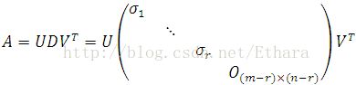
Any m-by-n matrix can be decomposed into

where U’s columns are the eigenvectors of AA^T, V’s columns are the eigenvectors of A^TA and

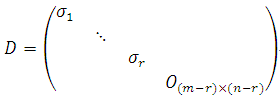
with sigma_i’s (1 <= i <= r) being the singular values of A.

Principal Component Analysis

Compared with factor analysis based on a probabilistic model and resorting to the iterative EM algorithm, PCA is known as a dimension reduction method, trying to directly identify the subspace in which the data approximately lies.

Given a data set,

chances are that some attributes are almost correlated. What PCA does is to reduce n-dimensional data to k-dimensional. Prior to running PCA algorithm, we need first to pre-process the data to normalize its mean and variance to be zero and one respectively, as follows:

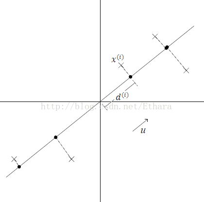
After having carried out this normalization, we might end up with a figure below.

How do we compute the “major axis of variation” u, that is, the direction on which the data approximately lies? One way to pose this problem is as finding the unit vector u so that when the data is projected onto the direction corresponding to u, the variance of the projected data is maximized. Intuitively, the data starts off with some amount of variance/information in it. We would like to choose a direction u so that if we were to approximate the data as lying in the direction/subspace corresponding to u, as much as possible of this variance is still retained.

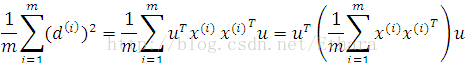
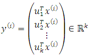
Noting that the length of the projection of x⁽ⁱ⁾ onto u is given by

we would like to choose a unit-length u to maximize the variance of all the projections,

Letting

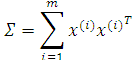
we pose the optimization problem to

Constructing Lagrange function,

Setting its derivative to zero,

we easily recognize that u must be the eigenvector of matrix SIGMA.

Noting that SIGMA is an n-by-n symmetric matrix having n independent eigenvectors, we should choose u₁,…,u_k to be the top k eigenvectors of SIGMA (the corresponding singular values must be in non-ascending order, for the optimization target equals to the eigenvalue) so as to project the data into a ­k-dimensional subspace (k < n).

By designing data matrix X,

and noting that (See the interpretation of matrix multiplication in Appendix)

we can efficiently compute top k eigenvectors u’s of data matrix X using SVD by X = UDV^T, since the top k columns of V are exactly the top k eigenvectors of X^TX = SIGMA. When x⁽ⁱ⁾ is high dimensional, X^TX would be much harder to represent. By computing V decomposed out of X, alternatively, the top k eigenvectors of X become available.

Since the top k eigenvectors of SIGMA have been determined, by projecting the data into this k-dimensional subspace, we can obtain the a new lower, k-dimensional approximation/representation for x⁽ⁱ⁾,

The vectors u₁,…,u_k are called the first k principal components of the data. Therefore, using SVD to implement PCA is a much better method if we are given a set of extremely high dimensional data.

Pseudo-inverse

Given an m-by-n matrix A whose rank is r, the two-sided inverse exists (AA^-1 = I = A^-1A) iff r = m = n (full rank).

In the case where r = n < m (n columns are independent <=> N(A) = {0}), the left inverse exists as A^-1_left = (A^TA)^-1A^T, for A^TA is always invertible. (See its proof in Appendix)

In the case where r = m < n (m rows are independent <=> N(A^T) = {0}), the right inverse exists as A^-1_right = A^T(AA^T)^-1, for AA^T is always invertible. (See its proof in Appendix)

In least squares, we have the projection matrix P_col = AA^-1_left = A(A^TA)^-1A^T which can project b onto the column space of A and the projection matrix P_row = A^-1_right A = A^T(AA^T)^-1A which can project b onto the row space of A.

However, for most of cases where r < min{m, n}, neither the left inverse nor the right inverse exists. How can we implement least square in this situation?

The pseudo-inverse denoted by A⁺ (n-by-m matrix) is the generalized inverse of A (m-by-n matrix) with any rank. Therefore, we can project b onto the column space of A by Pb, where P = AA⁺, and continue with the least squares.

SVD is an effective way to find the pseudo inverse A⁺ of A. First, decomposing A into

then, taking the pseudo-inverse of A, we obtain,

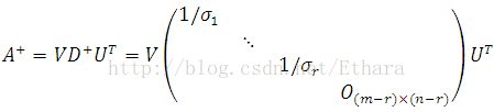
In conclusion, we can use SVD to find the pseudo-inverse of any matrix A whatsoever.

Appendix

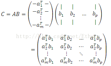
1. There are four ways to interpret the matrix multiplication (matrix-matrix product).

First, the most obvious viewpoint following immediately from the definition of matrix multiplication by representing A by rows and B by columns, symbolically, looks like the following.

Second, alternatively, we can represent A by columns and B by rows. This representation leads to a much trickier interpretation of AB as a sum of outer products. Symbolically,

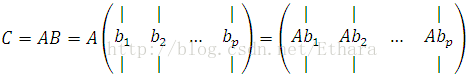
Third, we can view matrix-matrix product as a set of products between matrix and column vectors.

Fourth, we have the analogous viewpoint, where we represent A by rows, and view the rows of C as a set of products between row vectors and matrix. Symbolically,

2. A^TA is always invertible iff r = n < m (r is the rank of the m-by-n matrix A).

    Proof:

      A^TA (n-by-n matrix) is invertible <=> r(A^TA)= n <=>

      Equation A^TAx = 0 has only one solution x = 0 <=>

      (Ax)^T(Ax)= 0 has only one solution x = 0 <=>

      Ax = 0 has only one solution x = 0 <=> r(A) = n.

   Similarly, we can prove that AA^T is always invertible iff r = m < n.

Postscript

This is the last blog of the year 2014 during which everything finally worked out but Eth(...)ara. This work is for the loving memories of us.