Extensible Hashing

Extensible Hashing (Author: Marshall Schmitz, student, UW Oshkosh)

Objectives

• To understand how extensible hashing works

The Algorithm

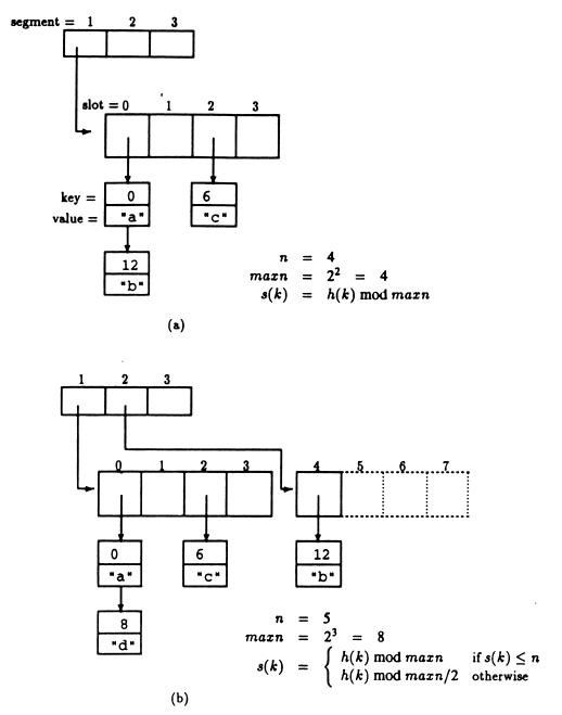
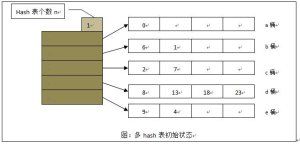
Extensible hashing is a form of dynamic hashing.  It has the advantages that static hashing has in that it can access data in constant time without searching through an entire database.  Additionally, extensible hashing does not have the drawbacks of static hashing.  With static hashing as the database grows in size it becomes more difficult to find places to put the data.  But with extensible hashing as the database fills up, the directory expands negating this problem.  Conversly, if the database shrinks in size, the directory shrinks and saves space in the process. 
 

Here is what the visualization looks like when it is first initalized.

 
 

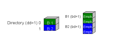
In the beginning of the algorithm, we start out with our two storage areas:  the directory and the buckets.

 
 

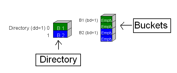
The directory has a property associated with it called the directory depth (abbreviated as dd) and each bucket has a property associated with it called the bucket depth (abbreviated as bd).

 
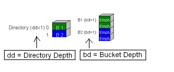
The directory is an array of pointers to buckets.  The color code scheme is used to indicate which bucket each directory element points at.

Three primary operations done on a hash table are: Add an element, Remove an element, and Search for an element.  Regardless of which operations are being done, the first steps are always the same.  First, the element to be inserted is sent to a hash function that returns a bit string.  From this bit string ,we look at the most significant dd bits to obtain the directory element.  Once we have the directory element we then load into memory the bucket that it references.

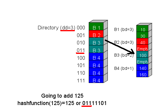
In this example we are performing an operation on 125.  When we send the value 125 to the hash function it returns  01111101.  Since the directory depth is 3, we look at the most significant 3 bits to obtain the directory element 011.  Directory element 011 points to bucket B3.  This is the bucket that needs to be loaded into memory. 
 

Searching for an Element:

With the bucket loaded into memory, it is searched for the element we are looking for.  If element is found in the bucket, then the element exists in the database; otherwise it does not exist.


Adding an Element

If the bucket is not full, then the element we are adding is placed in an available location.

If the bucket is full, then a new bucket is created and a Bucket Split is performed

A new bucket depth is given to both of these buckets.  It is equal to the number of most significant bits that all of these elements, including the element being added, share in common plus 1.

The elements in the full bucket are redistributed between the current bucket the elements are located in and the new bucket created.  If their most significant bd  bit is 0 then the element stays where it is; otherwise if the most signficant bd bit is 1 then this element is moved to the new bucket created.

If the new bd becomes larger than the directory depth then the directory depth must be changed to the bucket depth of this bucket and then the directory size must be expanded to 2 raised to the "new directory depth"th power

The pointers in the directory need to be adjusted.  In my coding I adjusted the pointers in a similar mannerly as demonstrated in this video at google videos:  Click Here To Watch This Video

Removing an Element 
 
• If the element is in the bucket, then remove this element from the bucket otherwise no other operations need to be performed
• If the bucket is not empty after removal of the element, then no other operations need to be performed.
• If the bucket is empty after removal of the element, then the bucket is to be deleted and a Bucket Merge is performed

  The pointers that used to point to this bucket are now pointed to the bucket it has  merged to.

  The bucket depth of the merged bucket is decreased until every element of the directory on the (bd)th most significant bits of the directory addresses don't point to this merged bucket

  If all of the bucket depths of each bucket are now smaller than the directory depth, then the directory depth must be changed to the largest bucket depth available and then the directory size must be shrunk to 2 raised to the power of the new directory depth.

  The pointers in the directory need to be adjusted.  Again I used the same method for readjustement as demonstrated in the google video.

转]动态哈希(dynamic hashing)  

        动态哈希表通常是在发生冲突后slot数量翻倍增长，而增长后毕竟哈希函数也变了，所以还要把旧slot里的元素重新放置。这种简单的动态哈希(dynamic hash)算法便是SGI版的STL中hash_map的实现。但如果每次调整slot都要全部重放元素，效率太低，且数据插入的时间也太不均匀：某次插入元素，发生了冲突，于是所有元素重新放置，老半天后这个元素才能插入完毕。作为实时系统，这一突如其来的延时当然是不可忍受的。
        为了让数据更新的时间更为均匀，数据库大师Per-Ake Larson便提出了一种新的动态哈希算法，其实中心思想也很简单（“简单是可靠的前提”——Dijkstra）：每次slot数量增长一倍，不是重新放置所有slot中的元素，而只移动一个slot内的元素——就是新增slot的那个兄弟slot（Buddy Slot）。如下：

slot增长前如图a，key为0、6的元素都可以放得下，但当key为12的元素到来时，编号为1的slot里有冲突了，这时需要将slot数翻一倍了，于是变成了图b。此时slot数由原来的4变为了现在的8，但“有效的”slot只有5个：编号分别为0到4。key为12的元素放入4号slot，因为12除8余4。按照一般的Larson策略来讲，4号slot的“兄弟slot”是0号slot，所以在增长完成后0号slot里所有除8余4的元素都要移到“新slot”即4号slot里，举个例子：如果0号slot里有key为16、20、24、28的元素，那key为20、28的元素必须移到4号slot，其它的（16和24）留在0号slot。
        只更新一个slot的代价是——查询要稍微复杂些：先用8去除key，如果余数对应的slot“不存在”，则再用4去除，得到正确的slot编号。例如查询6，先 6 mod 8 得6，6号slot还不存在（只是分配了内存，数据结构上还不存在），所以只能再除4，得2，到2号slot去找，找到。图b右下方的公式可能有一些误导：它通过看s(k)是否小于n(<=5)来判断对应的slot是否存在，而在通常的情况下，增长的slot可能不是4号。假如增长的是6号，这时4、5、7号slot是“不存在”的，再用这个公式硬套就不行了。所以关键的判断标准是slot“是否存在”，而不是编号本身是大是小。
        Per-Ake Larson的这一经典动态哈希算法以一小点查询时间的损失换来了数据更新的高效和平滑，因此得到了广泛的使用：GNU的gdbm、Berkeley的ndbm、雅虎的mdbm，都是使用这个算法。

E动态hash方法之一 
　　
　　动态hash方法之一
　　本文将介绍三种动态hash方法。
　　散列是一个非常有用的、非常基础的数据结构，在数据的查找方面尤其重要，应用的非常广泛。然而，任何事物都有两面性，散列也存在缺点，即数据的局部集中性会使散列的性能急剧下降，且越集中，性能越低。
　　数据集中，即搜索键在通过hash函数运算后，得到同一个结果，指向同一个桶，这时便产生了数据冲突。
　　通常解决数据冲突的方法有：拉链法(open hashing)和开地址法(open addressing)。拉链法我们用的非常多，即存在冲突时，简单的将元素链在当前桶的最后元素的尾部。开放地址法有线性探测再散列、二次线性探测再散列、再hash等方法。
　　以上介绍的解决冲突的方法，存在一个前提：hash表(又称散列表)的桶的数目保持不变，即hash表在初始化时指定一个数，以后在使用的过程中，只允许在其中添加、删除、查找元素等操作，而不允许改变桶的数目。
　　在实际的应用中，当hash表较小，元素个数不多时，采用以上方法完全可以应付。但是，一旦元素较多，或数据存在一定的偏斜性(数据集中分布在某个桶上)时，以上方法不足以解决这一问题。我们引入一种称之为动态散列的方法：在hash表的元素增长的同时，动态的调整hash桶的数目。
　　动态hash不需要对hash表中所有元素进行再次插入操作(重组)，而是在原来基础上，进行动态的桶扩展。有多种方法可以实现：多hash表、可扩展的动态散列和线性散列，下面分别介绍之，方法由简单到复杂。
　　多hash表：顾名思义，即采用多个hash表的方式扩展原hash表。这种方式不复杂，且理解起来也较简单，是三者中最简单的一种。
　　通常，当一个hash表冲突较多时，需要考虑采用动态hash方式，来减小后续操作继续在该桶上的冲突，减轻该桶负担，最简单且最容易想到的就是采用多hash表的方式。如下图，有一个简单的hash结构：
　　
　　简单起见，假定(1)hash函数采用模5，即hash(i)=i%5；(2)每个桶中最多只可放4个元素。
　　在以上基础上，向hash表中插入5，由于桶a存在空闲，直接存入。接着向hash表插入值3，由于d桶中已满，无空闲位置，此时在建立一个hash表，结果如下图
　　
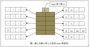
　　通过图示，一目了然，原来的一个hash表，变为现在的两个hash表。如需要，该“分裂”可继续进行。
　　需要注意的是：采用这种方式，多个hash表公用一个hash函数，且目录项的个数也随之增多，分别指向对应的桶。实际上，这时存在两个不同的目录项，分别指向各自的桶。
　　执行插入、查找、删除操作时，均需先求得hash值x。插入时，得到当前的hash表的个数，并分别取得各个目录项的x位置上的目录项，若其中某个项指向的桶存在空闲位置，则插入之。同时，在插入时，可保持多个hash表在某个目录项上桶中元素的个数近似相等。若不存在空闲位置，则简单的进行“分裂”，新建一个hash表，如上图所示。
　　查找时，由于某个记录值可能存在当前hash结构的多个表中，因此需同时在多个目录项的同一位置上进行查找操作，等待所有的查找结束后，方可判定该元素是否存在。由于该种结构需进行多次查找，当表元素非常多时，为提高效率，在多处理器上可采用多线程，并发执行查找操作。
　　删除操作，与上述过程基本类似，不赘述。需要注意的是，若删除操作导致某个hash表元素为空，这时可将该表从结构中剔除。
　　这

f

 

动态hash方法之二

 

线性散列：动态hash常用的另一种方法为线性散列，它能随数据的插入和删除，适当的对hash桶数进行调整，与可扩展散列相比，线性散列不需要存放数据桶指针的专门目录项，且能更自然的处理数据桶已满的情况，允许更灵活的选择桶分裂的时机，因此实现起来相比前两种方法要复杂。

      理解线性散列，需要引入“轮转分裂进化”的概念，各个桶轮流进行分裂，当一轮分裂完成之后，进入下一轮分裂，于是分裂将从头开始。用Level表示当前的“轮数”，其值从0开始。假定hash表初始桶数为N(要求N是2的幂次方)，则值logN(以2为底)是指用于表示N个数需要的最少二进制位数，用d0表示，即d0=logN。

      以上提到，用Level表示当前轮数，则每轮的初始桶数为N*2^Level个(2^Level表示2的Level次方)。例如当进行第0轮时，level值为0，则初始桶数为N*2^0=N。桶将按桶编号从小到大的顺序，依次发生分裂，一次分裂一个桶，这里我们使用Next指向下次将被分裂的桶。

      每次桶分裂的条件可灵活选择，例如，可设置一个桶的填充因子r(r<1)，当桶中记录数达到该值时进行分裂；也可选择当桶满时才进行分裂。

      需要注意的时，每次发生分裂的桶总是由Next决定，与当前值被插入的桶已满或溢出无关。为处理溢出情况，可引入溢出页解决。话不多说，先来看一个图示：

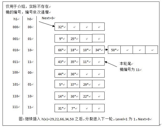
假定初始时，数据分布如上，hash函数为h(x)。桶数N=4，轮数Level为0，Next处于0位置；采用“发生溢出分裂”作为触发分裂的条件。此时d=logN=2，即使用两个二进位可表示桶的全部编号。

      简单解释一下，为什么32*、25*、18*分别位于第一、二、三个桶中。因为h(x)=32=100000，取最后两个二进制位00，对应桶编号00；h(y)=25=11001,取最后两个二进制位01，对应桶编号01；h(z)=18=10010，最后两位对应桶编号10。

      接下来，向以上hash表中插入两个新项h(x1)=43和h(x2)=37，插入结果如下图所示：

我们来分析一下。当插入h(x1)=43=101011时，d值为2，因此取末尾两个二进制位，应插入11桶。由于该桶已满，故应增加溢出页，并将43*插入该溢出页内。由于触发了桶分裂，因此在Next=0位置上(注意不是在11桶上)，进行桶分裂，产生00桶的映像桶，映像桶的编号计算方式为N+Next=4+0=100，且将原来桶内的所有元素进行重新分配，Next值移向下一个桶。

      当插入h(x2)=37=100101时，d值仍为2，取末尾两个二进制位，应插入01桶，该桶中有空余空间，直接插入。

      分析到这里，读者应该基本了解了线性散列的分裂方式。我们发现，桶分裂是依次进行的，且后续产生的映像桶一定位于上一次产生的映像桶之后。

      读者不妨继续尝试插入h(x)=29,22,66,34,50，情况如下图所示，这里不再详细分析。

线性散列的查找操作，例如要查询h(x)=18,32,44。假定查询时，hash表状态为N=4，Level=0,Next=1，因此d值为2。

(1)   查找h(x)=18=10010，取末两位10，由于10位于Next=1和N=4之间，对用桶还未进行分裂，直接取10作为桶编号，在该桶中进行查找。

(2)   查找h(x)=32=10000，取末两位00，由于00不在Next=1和N=4之间，表示该桶已经分裂，再向前取一位，因此桶编号为000，在该桶中进行查找。

(3)   查找h(x)=44=101100，取末两位00，由于00不在Next=1和N=4之间，表示该桶已经分裂，再向前取一位，因此桶编号为100，在该桶中进行查找。

      线性散列的删除操作是插入操作的逆操作，若溢出块为空，则可释放。若删除导致某个桶元素变空，则Next指向上一个桶。当Next减少到0，且最后一个桶也是空时，则Next指向N/2 -1的位置，同时Level值减1。

      线性散列比可扩展动态散列更灵活，且不需要存放数据桶指针的专门目录项，节省了空间；但如果数据散列后分布不均匀，导致的问题可能会比可扩展散列还严重。

至此，三种动态散列方式介绍完毕。

 

附：对于多hash表和可扩展的动态散列，桶内部的组织，可采用(1)链式方法，一个元素一个元素的链接起来，则上例中的4表示最多只能链接4个这样的元素；也可采用(2)块方式，每个块中可放若干个元素，块与块之间链接起来，则上例中的4表示最多只能链接4个这样的块。

 

 转载请注明原处：http://hi.baidu.com/calrincalrin/blog/item/b51b1910c7629265cb80c413.html

 

参考书籍：高级数据库系统及其应用，谢兴生主编，清华大学出版社(北京)，2010.1  

ficiency

 

动态hash之linear Hash的实现和性能比较

分类： C/C++语法的学习 数据库相关 算法和数据结构学习 STL 2011-07-31 20:22  493人阅读  评论(0)  收藏  举报

insert iterator pair class parameters algorithm

 

linear hash

 

一，在介绍linear hash 之前，需要对动态hash和静态hash这两个概念做一下解释：

 

静态hash：是指在hashtable初始化得时候bucket的数目就已经确定了，当需要插入一个元素的时候，通过hash函数找到对应的bucket number，之后插入即可。不论用什么冲突解决方法，当插入的元素越来越多时，在这个hash表中查找元素的效率会变的越来越低。

动态hash：是指在hashtable的bucket的数目不是确定的，而是会根据插入元素的多少而实现动态的增减，当元素变多得时候，bucket会动态增加，这样就可以解决静态hash的查找效率低得问题。当元素变少得时候，bucket会动态减少，从而减少空间的浪费。linear hash就是一种动态hash。

 

二。linear hash实现.

对于hash操作，主要有insert, find, erase三个操作，下面对linear_hash的3个操作做一些解析：

1.       Find.

对于查找操作，目的是输入key值，找出对应的卫星数据的值，这一操作和其他hash操作一样。

 bool find(KeyType iKey, DataType& oData)

                    {

                             int lKey = hashfunc(iKey);



                             if(lKey < 0 || lKey >= numBucket) return false;

                             bucketIter iter = mhashTable[lKey].begin();

                             for(; iter != mhashTable[lKey].end(); iter ++)

                             {

                                      if(iter->first == iKey)

                                      {

                                                oData = iter->second;

                                                return true;

                                      }

                             }



                             return false;

                    }

 

2.       Insert操作。

对于插入操作，客户端程序输入key值和卫星数据，进行这一操作，会增加Linearhash中的元素个数numElement，当Linearhash的bucket负载（numElements/numBuckets）超过一定值，需要动态的增加Bucket数，增加一个bucket, 接着需要把一个特定的bucket上的element分一部分到这个new 的bucket上。

 

 bool insert(KeyType iKey, DataType& iData)

                    {

                             int lKey = hashfunc(iKey);

                             if(lKey < 0 || lKey >= numBucket) return false;



                             //把这个element插入到对应的bucket（mHashTable[lKey]）里面

                             mhashTable[lKey].push_back(make_pair(iKey, iData));

                             numElement ++;



                             //计算现在Container的负载= 现在的元素个数/bucket数目

                             double loadFctr = (double)numElement / numBucket;

                             //如果负载操作最大的负载数，那么需要做extend操作。

                             //目的是增加bucket数，接着均分bucket上得element

                             if(loadFctr >= maxloadfctr)

                             {

                                      Extend();

                             }

                             return true;

                    }



  void Extend()

                      {

                             //计算出需要被均分的bucket位置mhashTable[oldPos].

                             //计算出新的bucket位置mhashTable[newPos].

                               int oldpos = p;

                               int newpos = numBucket;

                               mhashTable.resize(++ numBucket);



               //接着调整Container的状态，

                             //当p增加到最大的maxp的值时，需要成倍的增加maxp数，同时p回归为0

                               p = p + 1;

                               if(p == maxp)

                               {

                                        maxp *= 2;

                                        p = 0;

                               }



                             //接下来把mhashtable[oldpos]这个bucket中的元素按照一定的规则分配到nhashTable[newPos]内，一部分会留在原来的mhashtable[oldpos]中

                               bucketIter iter = mhashTable[oldpos].begin();

                               for(; iter != mhashTable[oldpos].end(); )

                               {

                                        if(hashfunc(iter->first) == newpos)

                                        {

                                                  mhashTable[newpos].push_back(make_pair(iter->first, iter->second));

                                                  iter = mhashTable[oldpos].erase(iter);

                                        }

                                        else

                                                  iter ++;



                               }



                      }

3.       Erase操作

对于erase操作，客户端程序给定key值，要求contianer删除其中和key值相同的元素。同时需要减少numElement数，当Linearhash的bucket负载（numElements/numBuckets）减少到一定值，需要动态的减少Bucket数，减少一个bucket, 同时需要把这个减少的bucket中的所有元素还原到原来的oldBucket中。

 bool erase(KeyType iKey)

                    {

                             int lKey = hashfunc(iKey);

                             if(lKey < 0 || lKey >= numBucket) return false;

                             bool isfound = false;

                             //在mhashTable[lKey]这个bucket中查找这个lKey值

 bucketIter iter = mhashTable[lKey].begin();

                             for(; iter != mhashTable[lKey].end(); )

                             {

                                      if(iter->first == iKey)

                                      {

                                                iter = mhashTable[lKey].erase(iter);

                                                isfound = true;

                                                break;

                                      }

                                      else

                                      {

                                                iter ++;

                                      }

                             }



                             //如果找到了，需要减少numElement值，调增bucekt数

                             if(isfound)

                             {

                                      numElement --;

                                      double loadFctr = (double)numElement / numBucket;

                                      if(loadFctr <= minloadfctr && numBucket > FIRSTBUCKETS)

                                      {

                                                Shrink();

                                      }

                                      return true;



                             }



                             return false;

                    }

 void Shrink()

                      {

                             //调增状态

                              p--;

                              if(p < 0)

                              {

                                       maxp /= 2;

                                       p = maxp -1;

                              }



                             //把mhashtable[numBucekt-1]中的元素全部insert到mhashtable[p]这个bucket中，

                             //同时调增mhashtable的大小。

                              mhashTable[p].insert(mhashTable[p].end(), mhashTable[numBucket-1].begin(), mhashTable[numBucket-1].end());

                              mhashTable[numBucket - 1].clear();

                              mhashTable.resize(--numBucket);



                      }

 

三．于STL：：map和STLEXT：：hash_map做了一下性能比较。

 

测试结果如下：

Linearhash insert time consume: 160

Linearhash find time consume: 50

Linearhash erase time consume: 70

map insert time consume: 80

map find time consume: 40

map erase time consume: 110

hash_map insert time consume: 150

hash_map find time consume: 40

hash_map erase time consume: 2130