西瓜书 习题3.5 编程实现LDA
参照西瓜书的课后习题3.5的要求,参考了一些资料,简单地实现了一下LDA。
数据还是西瓜数据3.0a
代码和数据,都挂在了我的git上:https://github.com/qdbszsj/LDA
首先第一部分还是画一个散点图,这个跟上一个习题是一样的,此处不详细表述了。
然后是先用sklearn偷懒实现一下LDA,这里要注意下模型参数的选择,对于小数据一般选择lsqr,这里给出了官方的reference可以查一下。
之后是自己实现LDA的步骤详解:
u是均值向量,对于二分类问题,每个个体有两个属性值,因此均值向量求出来是2*2的矩阵,就是求一下平均数。然后根据西瓜书P61的公式3.33求出类内散度矩阵,这里注意一下是列向量乘以自己的转置,最后的类内散度矩阵(within-class scatter matrix)是2*2的,记为Sw。这里根据公式3.39,我们求出Sw的逆矩阵就可以了,然而这里我们不用np.linalg.inv()来求逆矩阵,而是要考虑到数值的稳定性,采用先用奇异值分解(SVD),再用分解出的矩阵得到一个类似原Sw的逆矩阵的东西,我不太明白这里为何要用SVD绕一圈,为何这样就增加了数值的稳定性?查阅了相关的资料,有说矩阵是相似的,特征值等比例缩放所以没关系,具体的说法也没搜到,通常都是一笔带过,不知道为何这里不能直接对Sw求逆矩阵,望dalao们指教一下。然后根据公式3.39我们就得到了w,也就是一条线的方向或者说是一个方向向量(x,y),把数据垂直映射到这条线上就行了。
import numpy as np # for matrix calculation
# load the CSV file as a numpy matrix
#separate the data with " "(blank,\t)
dataset = np.loadtxt('/home/parker/watermelonData/watermelon3_0a.csv', delimiter=",")
print(dataset)
# separate the data from the target attributes
X = dataset[:, 1:3]
y = dataset[:, 3]
goodData=dataset[:8]
badData=dataset[8:]
#return the size
m, n = np.shape(X)
#print(m,n)#17,2
# draw scatter diagram to show the raw data
#https://matplotlib.org/api/pyplot_summary.html
'''
LDA via sklearn
'''
from sklearn import model_selection
from sklearn.discriminant_analysis import LinearDiscriminantAnalysis
from sklearn import metrics
import matplotlib.pyplot as plt
# generalization of train and test set
X_train, X_test, y_train, y_test = model_selection.train_test_split(X, y, test_size=0.5, random_state=0)
# model fitting
#http://scikit-learn.org/stable/modules/generated/sklearn.discriminant_analysis.
# LinearDiscriminantAnalysis.html#sklearn.discriminant_analysis.LinearDiscriminantAnalysis
lda_model = LinearDiscriminantAnalysis(solver='lsqr', shrinkage=None).fit(X_train, y_train)
# model validation
y_pred = lda_model.predict(X_test)
# summarize the fit of the model
print(metrics.confusion_matrix(y_test, y_pred))
print(metrics.classification_report(y_test, y_pred))
f1 = plt.figure(1)
plt.title('watermelon_3a')
plt.xlabel('density')
plt.ylabel('ratio_sugar')
"""
plt.scatter(X[y == 0, 0], X[y == 0, 1], marker='o', color='b', s=100, label='bad')
"""
plt.scatter(goodData[:,1], goodData[:,2], marker='o', color='g', s=100, label='good')
plt.scatter(X[y == 0, 0], X[y == 0, 1], marker='o', color='k', s=100, label='bad')
plt.legend(loc='upper right')
'''
implementation of LDA based on self-coding
'''
u = [[badData[:,1].mean(),badData[:,2].mean()],[goodData[:,1].mean(),goodData[:,2].mean()]]
u=np.matrix(u)
Sw = np.zeros((n,n))
for i in range(m):
x_tmp = X[i].reshape(n,1) # row -> cloumn vector
if y[i] == 0: u_tmp = u[0].reshape(n,1)
if y[i] == 1: u_tmp = u[1].reshape(n,1)
Sw += np.dot( x_tmp - u_tmp, (x_tmp - u_tmp).T )
# print(Sw)
U, sigma, V= np.linalg.svd(Sw)
#https://docs.scipy.org/doc/numpy/reference/generated/numpy.diag.html
Sw_inv = V.T * np.linalg.inv(np.diag(sigma)) * U.T
# print(Sw_inv)
# print(np.linalg.inv(Sw))
# 3-th. computing the parameter w, refer on book (3.39)
w = np.dot( Sw_inv, (u[0] - u[1]).reshape(n,1) ) # here we use a**-1 to get the inverse of a ndarray
print(w)
# P=[]
# for i in range(2): # two class
# P.append(np.mean(X[y==i], axis=0)) # column mean
f3 = plt.figure(3)
plt.xlim( 0, 1 )
plt.ylim( 0, 0.7 )
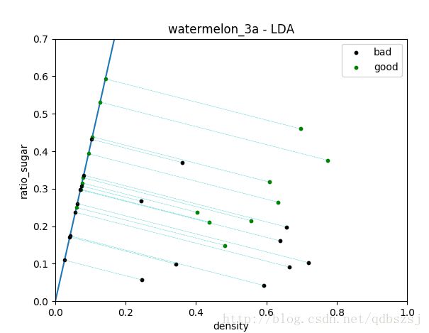
plt.title('watermelon_3a - LDA')
plt.xlabel('density')
plt.ylabel('ratio_sugar')
plt.scatter(X[y == 0,0], X[y == 0,1], marker = 'o', color = 'k', s=10, label = 'bad')
plt.scatter(X[y == 1,0], X[y == 1,1], marker = 'o', color = 'g', s=10, label = 'good')
plt.legend(loc = 'upper right')
k=w[1,0]/w[0,0]
plt.plot([-1,1], [-k, k])
for i in range(m):
curX=(k*X[i,1]+X[i,0])/(1+k*k)
if y[i]==0:plt.plot(curX,k*curX,"ko",markersize=3)
else:plt.plot(curX,k*curX,"go",markersize=3)
plt.plot([curX,X[i,0]],[k*curX,X[i,1]],"c--",linewidth=0.3)
plt.show() 
参考资料:
周志华《机器学习》P60-63
大犇git:https://github.com/PY131/Machine-Learning_ZhouZhihua/blob/master/ch3_linear_model/3.5_LDA/src/LDA.py