- 2025年网络安全人员薪酬趋势
程序员肉肉
web安全安全网络安全计算机信息安全程序员
2025年网络安全人员薪酬趋势一、网络安全行业为何成“香饽饽”?最近和几个朋友聊起职业规划,发现一个有趣的现象:不管原来是程序员、运维还是产品经理,都想往网络安全领域跳槽。问原因,答案出奇一致——“听说这行工资高”。确实,从2025年的数据来看,网络安全行业的薪资水平不仅跑赢了大多数IT岗位,甚至成了“技术岗里的天花板”。但高薪背后到底有哪些门道?哪些职位最赚钱?城市和经验如何影响收入?今天我们就
- 搜广推校招面经九十三
Y1nhl
搜广推面经机器学习人工智能python算法推荐算法pytorch搜索算法
字节懂车帝一面一、NDCG(NormalizedDiscountedCumulativeGain)的计算NDCG是信息检索和排序任务中常用的评价指标,用于衡量模型预测的排序质量与真实相关性排序的一致程度。1.1.DCG@k(DiscountedCumulativeGain)DCG@k=∑i=1krelilog2(i+1)\text{DCG@k}=\sum_{i=1}^{k}\frac{rel_i
- windows exe爬虫:exe抓包
程序猿阿三
爬虫项目实战exe抓包
不论任何爬虫,抓包是获取数据最直接和最方便的方式,这章节我们一起看一下windowsexe是如何拦截数据的。用mitmproxy/Charles/Fiddler或Wireshark拦截它的HTTP/HTTPS/TCP流量。如果是HTTPS,安装并信任代理的根证书。由于exe大部分可能走的是自定义应用层协议。在不知情所拦截应用使用的流量时,所以建议用Wireshark。本文利用python代码,实现
- PythonDay01
这里写目录标题一、注释1、单行注释2、多行注释二、定义变量1、要求2、代码三、关键字四、print函数五、基本数据类型1、整型2、字符串类型3、小数类型4、布尔类型5、空类型六、类型之间的相互转换1、从字符串转成int类型2、字符串转换成浮点型3、float转换成int4、丢失精度时不会去做四舍五入5、布尔类型七、字符串的常见操作1、split切分2、strip去除字符串两边的隐藏字符3、字符串的
- Docker初识:mysql8主从复制(单向)- 主从搭建扩展知识
滴水可藏海
#mysql数据库
主从服务(master-slave)新学习到的知识。1、全库同步与部分同步上回书说到Docker初识:mysql8主从复制(单向)的配置都是针对全库配置的。但是实际上并不需要针对全库做备份,只需要对一些特别重要的库或者表来进行同步。例如information_schema等。可以通过配置文件中的一些属性指定需要针对哪些库或者哪些表记录binlog。Master配置:#需要同步的二进制数据库名bin
- 【AI大模型】LLM模型架构深度解析:BERT vs. GPT vs. T5
我爱一条柴ya
学习AI记录ai人工智能AI编程python
引言Transformer架构的诞生(Vaswanietal.,2017)彻底改变了自然语言处理(NLP)。在其基础上,BERT、GPT和T5分别代表了三种不同的模型范式,主导了预训练语言模型的演进。理解它们的差异是LLM开发和学习的基石。一、核心架构对比特性BERT(BidirectionalEncoder)GPT(GenerativePre-trainedTransformer)T5(Text
- Python Day9
@浙大疏锦行PythonDay9.内容:热力图的绘制enumerate()方法子图的绘制代码:list_nums=[1,2,3,4,5,6]forindex,valinenumerate(list_nums):print(f"index={index},val={val}")forvalinlist_nums:print(f"val={val}")importpandasaspdimportmat
- mit6.s081lab
临近毕业季,回想自己本科四年学到了哪些东西,想到自己专业课都是为了卷绩点、应付考试,去背书、被概念,并没有十分深刻的理解和动手实践。现在想重新温习一下这部分知识,同时也加深一下对这部分内容的动手实践。那么就从大名鼎鼎的os课6.s081开始吧~~~lab1:Unixutilitieslab2:Systemcalls
- 【代码学习】扩散模型原理+代码
李加号pluuuus
CV基础代码学习扩散模型机器学习算法学习
来源:超详细的扩散模型(DiffusionModels)原理+代码-知乎(zhihu.com)代码:drizzlezyk/DDPM-MindSpore(github.com)DDPM1.Unet1.1正弦位置编码classSinusoidalPosEmb(nn.Cell):def__init__(self,dim):super().__init__()half_dim=dim//2#将给定的维度除
- 【医学影像】无痛安装mamba
周树皮
医学影像python
去年编辑的一个帖子。摆了一段时间后重新回归,发送一下作为状态分界线。很癫狂的体验,man,whatcanisay!issue查看我的狗急跳墙状态1.确定版本cudanvcc-Vpythonpython--versiontorchpipshowtorch2.下载对应版本wheelcausal-conv1d:https://github.com/Dao-AILab/causal-conv1d/rele
- Android 图像处理 - Bitmap 图像处理观察记录(基本图像复制、带目录创建的图像复制、字节流处理的图像复制、并发图像复制、单线程池顺序图像复制)
Bitmap图像处理观察记录1、基本图像复制从应用内部存储目录读取test.png使用BitmapFactory解码为Bitmap对象将Bitmap重新压缩保存为newTest.png操作成功,compress返回trueFilefile=newFile(getFilesDir(),"test.png");StringabsolutePath=file.getAbsolutePath();Bitm
- macd的python代码同花顺_同花顺最牛MACD副图源码
再来一碗饭
DIFF:EMA(CLOSE,6)-EMA(CLOSE,16),ColorFFFF26;DEA:EMA(DIFF,5),Color8A15FF;MACD:=2*(DIFF-DEA);对DIFF:0-(EMA(CLOSE,6)-EMA(CLOSE,16));对DEA:0-(EMA(DIFF,5));对称:0-(2*(DIFF-DEA)),STICK,ColorFF6060,LINETHICK1;{D
- Ollama平台里最流行的embedding模型: nomic-embed-text 模型介绍和实践
skywalk8163
人工智能embedding人工智能服务器
nomic-embed-text模型介绍nomic-embed-text是一个基于SentenceTransformers库的句子嵌入模型,专门用于特征提取和句子相似度计算。该模型在多个任务上表现出色,特别是在分类、检索和聚类任务中。其核心优势在于能够生成高质量的句子嵌入,这些嵌入在语义上非常接近,从而在相似度计算和分类任务中表现优异。之所以选用这个模型,是因为在Ollama网站查找这个模型,发现
- LLM 大模型学习必知必会系列(十三):基于SWIFT的VLLM推理加速与部署实战
汀、人工智能
LLM技术汇总人工智能自然语言处理LLMAgentvLLMAI大模型大模型部署
LLM大模型学习必知必会系列(十三):基于SWIFT的VLLM推理加速与部署实战1.环境准备GPU设备:A10,3090,V100,A100均可.#设置pip全局镜像(加速下载)pipconfigsetglobal.index-urlhttps://mirrors.aliyun.com/pypi/simple/#安装ms-swiftpipinstall'ms-swift[llm]'-U#vllm与
- 目标检测中的NMS算法详解
好的,我们来详细解释一下目标检测中非极大值抑制(Non-MaximumSuppression,NMS)的相关概念和计算过程。1.为什么需要NMS?问题:目标检测模型(如FasterR-CNN,YOLO,SSD等)在推理时,对于同一个目标物体,通常会预测出多个重叠的、不同置信度(confidencescore)的候选边界框(BoundingBoxes)。直接输出所有这些框会导致:结果冗余:同一个物体
- Unity物理系统由浅入深第二节:物理系统高级特性与优化
吉良吉影NeKoSuKi
unity游戏引擎架构c#开发语言
本次我们将简单讲解Unity物理系统的一些高级特性,例如物理层、各种关节、布料系统和车辆物理等,这些能够帮助我们理解复杂的物理模拟原理。同时,我们也会探讨物理系统的性能开销,并提供优化策略,确保我们的游戏在拥有丰富物理效果的同时,也能保持良好的帧率。1.物理层(PhysicsLayers):精细控制碰撞行为在大型或复杂的场景中,你可能不希望所有物体都相互碰撞。例如,玩家的子弹应该能击中敌人,但不应
- CMD,PowerShell、Linux/MAC设置环境变量
sky丶Mamba
零基础转大模型应用开发linuxmacos运维
以下是CMD(Windows)、PowerShell(Windows)、Linux/Mac在临时/永久环境变量操作上的对比表格:环境变量操作对照表(CMDvsPowerShellvsLinux/Mac)操作CMD(Windows)PowerShell(Windows)Linux/Mac(Bash/Zsh)设置临时变量setVAR=value$env:VAR="value"exportVAR=val
- 《手机摄影从实战到精通》——多个技能多条路,手机拍摄技巧,着实过分实用了
Ann2015
智能手机程序人生学习生活风景
用小小的一部手机,就能拍大片?是的,手机摄影已不容小觑。近年来,一些手机厂商邀请知名导演使用手机拍大片,以彰显手机性能的强大,这也重新定义了我们对手机摄影的认知。相较于传统摄影设备,智能手机自带的“计算摄影”性能也降低了拍摄门槛,它可以将原本需要手动调节的各项参数指标进行自动调整和优化,使我们能轻松获得最佳拍摄效果。这也大大降低了拍摄的难度和门槛,让我们将重点放在内容创作上。手机与视频平台也密不可
- Spring 如何干预 Bean 的生命周期?
冰糖心书房
SpringIOCIocspringBean生命周期
Spring提供了多种机制让我们能够在Bean生命周期的不同节点“插入”自己的逻辑,这些机制可以分为两大类:针对单个Bean的干预和针对所有/多个Bean的全局干预。一、针对单个Bean的干预(最常用)这些方法让你为一个特定的Bean类定义其初始化和销毁逻辑。1.使用JSR-250注解(推荐方式)这是现在最优雅、也是Spring官方推荐的方式。它使用Java的标准注解,与Spring框架解耦。@P
- Mysql字段没有索引,通过where x = 3 for update是使用什么级别的锁
没有索引时,FORUPDATE会锁住整个表现在,你正在一本一本地翻看所有书,寻找“维修中”的书,并且你对管理员说:“在我清点和修改完之前,别人不能动这些书,也不能往这个范围里加新书!”问题1:如何锁住你找到的“维修中”的书?你每找到一本“维修中”的书,就给它贴上一个“正在处理,请勿触碰”的标签(行级排他锁)。问题2:如何防止别人“往这个范围里加新书”?这是最关键的。因为你没有“状态”的目录卡片(没
- [论文阅读]Distilling Step-by-Step! Outperforming Larger Language Models with Less Training Data and Smal
0x211
论文阅读语言模型人工智能自然语言处理
中文译名:逐步蒸馏!以较少的训练数据和较小的模型规模超越较大的语言模型发布链接:http://arxiv.org/abs/2305.02301AcceptedtoFindingsofACL2023阅读原因:近期任务需要用到蒸馏操作,了解相关知识核心思想:改变视角。原来的视角:把LLMs视为噪声标签的来源。现在的视角:把LLMs视为能够推理的代理。方法好在哪?需要的数据量少,得到的结果好。文章的方法
- 在拉卡拉分账功能中实现实时更新,需结合异步回调通知和数据库事务来确保数据一致性。以下是具体实现方案
肥仔全栈开发
拉卡拉支付php拉卡拉支付三方支付
一、实时更新的核心逻辑依赖拉卡拉分账回调拉卡拉分账完成后会主动推送回调通知(类似支付回调),需监听该回调并更新订单分账状态。数据库事务保障分账金额更新、状态变更等操作需放在事务中,避免部分失败导致数据不一致。二、代码实现1.分账回调处理接口(监听拉卡拉分账结果推送,实时更新数据库)//文件:application/api/controller/Notify.phppublicfunctionlak
- 对接拉卡拉聚合收银台支付指南
一叶飘零_sweeeet
果酱紫javajava支付支付宝支付微信支付拉卡拉支付
今天我将详细介绍如何对接拉卡拉聚合收银台支付,并指出其中应注意的点。我希望这篇文章能够帮助那些正在寻找如何实现这个功能的开发者。一、拉卡拉聚合收银台支付简介拉卡拉聚合收银台支付是一种整合了多种支付方式的支付服务,包括但不限于微信支付、支付宝支付、银联支付等。它为商户提供了一个统一的支付入口,使得商户无需分别接入各种支付方式,从而大大简化了支付过程。二、对接拉卡拉聚合收银台支付的步骤1.注册并配置拉
- Mamba项目用户指南:高效管理Python环境的利器
左松钦Travis
Mamba项目用户指南:高效管理Python环境的利器mambaTheFastCross-PlatformPackageManager项目地址:https://gitcode.com/gh_mirrors/mam/mamba什么是Mamba?Mamba是一个基于Conda的CLI工具,专为高效管理Python环境而设计。它继承了Conda的所有优点,同时在性能上进行了显著优化,特别是在解决依赖关系
- 【亲测免费】 Mamba:快速跨平台的包管理器
林梦雅
Mamba:快速跨平台的包管理器项目基础介绍和主要编程语言Mamba是一个用C++重新实现的Conda包管理器。它旨在提供比传统Conda更快的包管理和依赖解析速度。Mamba的核心部分使用C++编写,以确保高效性和性能。同时,Mamba也使用了Python和其他一些辅助语言来实现其功能。项目核心功能Mamba的核心功能包括:快速依赖解析:利用libsolv库进行高效的依赖解析,这是RedHat、
- 【Modern C++ Part8】Prefer-nullptr-to-0-and-NULL
莫彩
C++ModernC++c++开发语言jvm
优先使用nullptr而不是0或者NULL0字面上是一个int类型,而不是指针,这是显而易见的。C++扫描到一个0,但是发现在上下文中仅有一个指针用到了它,编译器将勉强将0解释为空指针,但是这仅仅是一个应变之策。C++最初始的原则是0是int而非指针。经验上讲,同样的情况对NULL也是存在的。对NULL而言,仍有一些细节上的不确定性,因为赋予NULL一个除了int(即long)以外的整数类型是被允
- 【Modern C++ Part7】_创建对象时使用()和{}的区别
莫彩
ModernC++C++c++开发语言
在C++11中,你可以有多种语法选择用以对象的初始化,这样的语法显得混乱不堪并让人无所适从,(),=,{}均可以用来进行初始化:intx(0);//使用()进行初始化inty=0;//使用=进行初始化intz{0};//使用{}进行初始化在很多情况下,可以同时使用=和{}intz={0};//使用{}和=进行初始化对于这一条,我通常的会忽略“等于-{}”这种语法,因为C通常认为它只有{}。认为这种
- 2025年的RAG技术发展趋势与演进
码农Q!
云计算人工智能aiagi自然语言处理语言模型
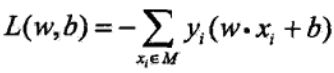
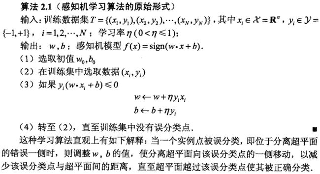
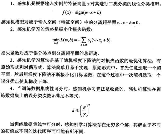
本文将分享作为大模型应用创业者的经历与观察,讨论RAG技术和市场环境在2024年的变化。一、RAG技术的演进RAG(检索增强生成)由“检索”和“大模型生成”两部分组成,而检索之前的索引创建(如chunking、embedding等)是核心基础。我们早在2021年便通过Java技术栈实现了RAG的“RA”部分。2023年中,RAG概念突然走红,并迅速在企业应用中显示出更强的实用性。1.主流架构的变化
- GPT实操——利用GPT创建一个应用
狗木马
深度学习gpt-3gpt
功能描述信息查询:用户可以询问各种问题,如天气、新闻、股票等,机器人会返回相关信息。任务执行:用户可以要求机器人执行一些简单的任务,如设置提醒、发送邮件等。情感支持:机器人可以与用户进行情感交流,提供安慰和支持。个性化设置:用户可以自定义机器人的回复风格和偏好。技术栈前端:React.js后端:Node.js+Express数据库:MongoDB自然语言处理:OpenAIGPT-3API其他工具:
- Android开发中RxJava的使用与原理
你过来啊你
androidrxjava
RxJava是ReactiveExtensions在JVM上的实现,专为处理异步事件流和基于观察者模式的编程而设计。在Android开发中,它极大地简化了异步操作(如网络请求、数据库访问、UI事件处理)的管理、组合和线程调度,有效解决了回调地狱问题。一、RxJava核心概念Observable(可观察者):数据源或事件源。它负责发出数据项(onNext)或事件(成功完成onComplete/发生错
- 戴尔笔记本win8系统改装win7系统
sophia天雪
win7戴尔改装系统win8
戴尔win8 系统改装win7 系统详述
第一步:使用U盘制作虚拟光驱:
1)下载安装UltraISO:注册码可以在网上搜索。
2)启动UltraISO,点击“文件”—》“打开”按钮,打开已经准备好的ISO镜像文
- BeanUtils.copyProperties使用笔记
bylijinnan
java
BeanUtils.copyProperties VS PropertyUtils.copyProperties
两者最大的区别是:
BeanUtils.copyProperties会进行类型转换,而PropertyUtils.copyProperties不会。
既然进行了类型转换,那BeanUtils.copyProperties的速度比不上PropertyUtils.copyProp
- MyEclipse中文乱码问题
0624chenhong
MyEclipse
一、设置新建常见文件的默认编码格式,也就是文件保存的格式。
在不对MyEclipse进行设置的时候,默认保存文件的编码,一般跟简体中文操作系统(如windows2000,windowsXP)的编码一致,即GBK。
在简体中文系统下,ANSI 编码代表 GBK编码;在日文操作系统下,ANSI 编码代表 JIS 编码。
Window-->Preferences-->General -
- 发送邮件
不懂事的小屁孩
send email
import org.apache.commons.mail.EmailAttachment;
import org.apache.commons.mail.EmailException;
import org.apache.commons.mail.HtmlEmail;
import org.apache.commons.mail.MultiPartEmail;
- 动画合集
换个号韩国红果果
htmlcss
动画 指一种样式变为另一种样式 keyframes应当始终定义0 100 过程
1 transition 制作鼠标滑过图片时的放大效果
css
.wrap{
width: 340px;height: 340px;
position: absolute;
top: 30%;
left: 20%;
overflow: hidden;
bor
- 网络最常见的攻击方式竟然是SQL注入
蓝儿唯美
sql注入
NTT研究表明,尽管SQL注入(SQLi)型攻击记录详尽且为人熟知,但目前网络应用程序仍然是SQLi攻击的重灾区。
信息安全和风险管理公司NTTCom Security发布的《2015全球智能威胁风险报告》表明,目前黑客攻击网络应用程序方式中最流行的,要数SQLi攻击。报告对去年发生的60亿攻击 行为进行分析,指出SQLi攻击是最常见的网络应用程序攻击方式。全球网络应用程序攻击中,SQLi攻击占
- java笔记2
a-john
java
类的封装:
1,java中,对象就是一个封装体。封装是把对象的属性和服务结合成一个独立的的单位。并尽可能隐藏对象的内部细节(尤其是私有数据)
2,目的:使对象以外的部分不能随意存取对象的内部数据(如属性),从而使软件错误能够局部化,减少差错和排错的难度。
3,简单来说,“隐藏属性、方法或实现细节的过程”称为——封装。
4,封装的特性:
4.1设置
- [Andengine]Error:can't creat bitmap form path “gfx/xxx.xxx”
aijuans
学习Android遇到的错误
最开始遇到这个错误是很早以前了,以前也没注意,只当是一个不理解的bug,因为所有的texture,textureregion都没有问题,但是就是提示错误。
昨天和美工要图片,本来是要背景透明的png格式,可是她却给了我一个jpg的。说明了之后她说没法改,因为没有png这个保存选项。
我就看了一下,和她要了psd的文件,还好我有一点
- 自己写的一个繁体到简体的转换程序
asialee
java转换繁体filter简体
今天调研一个任务,基于java的filter实现繁体到简体的转换,于是写了一个demo,给各位博友奉上,欢迎批评指正。
实现的思路是重载request的调取参数的几个方法,然后做下转换。
- android意图和意图监听器技术
百合不是茶
android显示意图隐式意图意图监听器
Intent是在activity之间传递数据;Intent的传递分为显示传递和隐式传递
显式意图:调用Intent.setComponent() 或 Intent.setClassName() 或 Intent.setClass()方法明确指定了组件名的Intent为显式意图,显式意图明确指定了Intent应该传递给哪个组件。
隐式意图;不指明调用的名称,根据设
- spring3中新增的@value注解
bijian1013
javaspring@Value
在spring 3.0中,可以通过使用@value,对一些如xxx.properties文件中的文件,进行键值对的注入,例子如下:
1.首先在applicationContext.xml中加入:
<beans xmlns="http://www.springframework.
- Jboss启用CXF日志
sunjing
logjbossCXF
1. 在standalone.xml配置文件中添加system-properties:
<system-properties> <property name="org.apache.cxf.logging.enabled" value=&
- 【Hadoop三】Centos7_x86_64部署Hadoop集群之编译Hadoop源代码
bit1129
centos
编译必需的软件
Firebugs3.0.0
Maven3.2.3
Ant
JDK1.7.0_67
protobuf-2.5.0
Hadoop 2.5.2源码包
Firebugs3.0.0
http://sourceforge.jp/projects/sfnet_findbug
- struts2验证框架的使用和扩展
白糖_
框架xmlbeanstruts正则表达式
struts2能够对前台提交的表单数据进行输入有效性校验,通常有两种方式:
1、在Action类中通过validatexx方法验证,这种方式很简单,在此不再赘述;
2、通过编写xx-validation.xml文件执行表单验证,当用户提交表单请求后,struts会优先执行xml文件,如果校验不通过是不会让请求访问指定action的。
本文介绍一下struts2通过xml文件进行校验的方法并说
- 记录-感悟
braveCS
感悟
再翻翻以前写的感悟,有时会发现自己很幼稚,也会让自己找回初心。
2015-1-11 1. 能在工作之余学习感兴趣的东西已经很幸福了;
2. 要改变自己,不能这样一直在原来区域,要突破安全区舒适区,才能提高自己,往好的方面发展;
3. 多反省多思考;要会用工具,而不是变成工具的奴隶;
4. 一天内集中一个定长时间段看最新资讯和偏流式博
- 编程之美-数组中最长递增子序列
bylijinnan
编程之美
import java.util.Arrays;
import java.util.Random;
public class LongestAccendingSubSequence {
/**
* 编程之美 数组中最长递增子序列
* 书上的解法容易理解
* 另一方法书上没有提到的是,可以将数组排序(由小到大)得到新的数组,
* 然后求排序后的数组与原数
- 读书笔记5
chengxuyuancsdn
重复提交struts2的token验证
1、重复提交
2、struts2的token验证
3、用response返回xml时的注意
1、重复提交
(1)应用场景
(1-1)点击提交按钮两次。
(1-2)使用浏览器后退按钮重复之前的操作,导致重复提交表单。
(1-3)刷新页面
(1-4)使用浏览器历史记录重复提交表单。
(1-5)浏览器重复的 HTTP 请求。
(2)解决方法
(2-1)禁掉提交按钮
(2-2)
- [时空与探索]全球联合进行第二次费城实验的可能性
comsci
二次世界大战前后,由爱因斯坦参加的一次在海军舰艇上进行的物理学实验 -费城实验
至今给我们大家留下很多迷团.....
关于费城实验的详细过程,大家可以在网络上搜索一下,我这里就不详细描述了
在这里,我的意思是,现在
- easy connect 之 ORA-12154: TNS: 无法解析指定的连接标识符
daizj
oracleORA-12154
用easy connect连接出现“tns无法解析指定的连接标示符”的错误,如下:
C:\Users\Administrator>sqlplus username/
[email protected]:1521/orcl
SQL*Plus: Release 10.2.0.1.0 – Production on 星期一 5月 21 18:16:20 2012
Copyright (c) 198
- 简单排序:归并排序
dieslrae
归并排序
public void mergeSort(int[] array){
int temp = array.length/2;
if(temp == 0){
return;
}
int[] a = new int[temp];
int
- C语言中字符串的\0和空格
dcj3sjt126com
c
\0 为字符串结束符,比如说:
abcd (空格)cdefg;
存入数组时,空格作为一个字符占有一个字节的空间,我们
- 解决Composer国内速度慢的办法
dcj3sjt126com
Composer
用法:
有两种方式启用本镜像服务:
1 将以下配置信息添加到 Composer 的配置文件 config.json 中(系统全局配置)。见“例1”
2 将以下配置信息添加到你的项目的 composer.json 文件中(针对单个项目配置)。见“例2”
为了避免安装包的时候都要执行两次查询,切记要添加禁用 packagist 的设置,如下 1 2 3 4 5
- 高效可伸缩的结果缓存
shuizhaosi888
高效可伸缩的结果缓存
/**
* 要执行的算法,返回结果v
*/
public interface Computable<A, V> {
public V comput(final A arg);
}
/**
* 用于缓存数据
*/
public class Memoizer<A, V> implements Computable<A,
- 三点定位的算法
haoningabc
c算法
三点定位,
已知a,b,c三个顶点的x,y坐标
和三个点都z坐标的距离,la,lb,lc
求z点的坐标
原理就是围绕a,b,c 三个点画圆,三个圆焦点的部分就是所求
但是,由于三个点的距离可能不准,不一定会有结果,
所以是三个圆环的焦点,环的宽度开始为0,没有取到则加1
运行
gcc -lm test.c
test.c代码如下
#include "stdi
- epoll使用详解
jimmee
clinux服务端编程epoll
epoll - I/O event notification facility在linux的网络编程中,很长的时间都在使用select来做事件触发。在linux新的内核中,有了一种替换它的机制,就是epoll。相比于select,epoll最大的好处在于它不会随着监听fd数目的增长而降低效率。因为在内核中的select实现中,它是采用轮询来处理的,轮询的fd数目越多,自然耗时越多。并且,在linu
- Hibernate对Enum的映射的基本使用方法
linzx0212
enumHibernate
枚举
/**
* 性别枚举
*/
public enum Gender {
MALE(0), FEMALE(1), OTHER(2);
private Gender(int i) {
this.i = i;
}
private int i;
public int getI
- 第10章 高级事件(下)
onestopweb
事件
index.html
<!DOCTYPE html PUBLIC "-//W3C//DTD XHTML 1.0 Transitional//EN" "http://www.w3.org/TR/xhtml1/DTD/xhtml1-transitional.dtd">
<html xmlns="http://www.w3.org/
- 孙子兵法
roadrunners
孙子兵法
始计第一
孙子曰:
兵者,国之大事,死生之地,存亡之道,不可不察也。
故经之以五事,校之以计,而索其情:一曰道,二曰天,三曰地,四曰将,五
曰法。道者,令民于上同意,可与之死,可与之生,而不危也;天者,阴阳、寒暑
、时制也;地者,远近、险易、广狭、死生也;将者,智、信、仁、勇、严也;法
者,曲制、官道、主用也。凡此五者,将莫不闻,知之者胜,不知之者不胜。故校
之以计,而索其情,曰
- MySQL双向复制
tomcat_oracle
mysql
本文包括:
主机配置
从机配置
建立主-从复制
建立双向复制
背景
按照以下简单的步骤:
参考一下:
在机器A配置主机(192.168.1.30)
在机器B配置从机(192.168.1.29)
我们可以使用下面的步骤来实现这一点
步骤1:机器A设置主机
在主机中打开配置文件 ,
- zoj 3822 Domination(dp)
阿尔萨斯
Mina
题目链接:zoj 3822 Domination
题目大意:给定一个N∗M的棋盘,每次任选一个位置放置一枚棋子,直到每行每列上都至少有一枚棋子,问放置棋子个数的期望。
解题思路:大白书上概率那一张有一道类似的题目,但是因为时间比较久了,还是稍微想了一下。dp[i][j][k]表示i行j列上均有至少一枚棋子,并且消耗k步的概率(k≤i∗j),因为放置在i+1~n上等价与放在i+1行上,同理