【论文学习】Bidirectional LSTM-CRF Models for Sequence Tagging（论文翻译）

Bidirectional LSTM-CRF Models for Sequence Tagging（论文翻译）

Abstract

In this paper, we propose a variety of Long Short-Term Memory (LSTM) based models for sequence tagging. These models include LSTM networks, bidirectional LSTM (BI-LSTM) networks, LSTM with a Conditional Random Field (CRF) layer (LSTM-CRF) and bidirectional LSTM with a CRF layer (BI-LSTM-CRF). Our work is the first to apply a bidirectional LSTM CRF (denoted as BI-LSTM-CRF) model to NLP benchmark sequence tagging data sets. We show that the BILSTM-CRF model can efficiently use both past and future input features thanks to a bidirectional LSTM component. It can also use sentence level tag information thanks to a CRF layer. The BI-LSTMCRF model can produce state of the art (or close to) accuracy on POS, chunking and NER data sets. In addition, it is robust and has less dependence on word embedding as compared to previous observations.

在本文中，本文提出了一系列基于长短期记忆（LSTM）的序列标注模型。这些模型包括LSTM，BI-LSTM，LSTM-CRF，BI-LSTM-CRF我们的工作是首次将双向的LSTM CRF(简称BI-LSTM-CRF)模型应用于NLP基准序列标记数据集。我们证明，由于双向LSTM组件，bilsm - crf模型可以有效地利用过去和未来的输入特性。由于CRF层，它还可以使用句子级别的标记信息。BI-LSTMCRF模型可以在POS、分块和NER数据集上产生最先进(或接近)的精度。此外，与以前的观测相比，该方法具有较强的鲁棒性，对嵌入词的依赖性较小。

1.Introduction

Sequence tagging including part of speech tagging (POS), chunking, and named entity recognition (NER) has been a classic NLP task. It has drawn research attention for a few decades. The output of taggers can be used for down streaming applications. For example, a named entity recognizer trained on user search queries can be utilized to identify which spans of text are products, thus triggering certain products ads. Another example is that such tag information can be used by a search engine to find relevant webpages.

序列标记包括词性标记(POS)、分块和命名实体识别(NER)，一直是经典的NLP任务。几十年来，它引起了研究界的关注。标记器的输出可以用于下行流应用程序。例如，一个在用户搜索查询上训练好的命名实体识别器，可以用来识别文本中的哪些词是产品，从而触发某些产品广告。另一个例子是，这样的标签信息可以被搜索引擎用来查找相关网页。

Most existing sequence tagging models are linear statistical models which include Hidden Markov Models (HMM), Maximum entropy Markov models (MEMMs) (McCallum et al., 2000), and Conditional Random Fields (CRF) (Lafferty et al., 2001). Convolutional network based models (Collobert et al., 2011) have been recently proposed to tackle sequence tagging problem. We denote such a model as Conv-CRF as it consists of a convolutional network and a CRF layer on the output (the term of sentence level loglikelihood (SSL) was used in the original paper). The Conv-CRF model has generated promising results on sequence tagging tasks. In speech language understanding community, recurrent neural network (Mesnil et al., 2013; Yao et al., 2014) and convolutional nets (Xu and Sarikaya, 2013) based models have been recently proposed. Other relevant work includes (Graves et al., 2005; Graves et al., 2013) which proposed a bidirectional recurrent neural network for speech recognition.

现有的序列标记模型大多是线性统计模型，包括隐马尔可夫模型(HMM)、最大熵马尔可夫模型(MEMMs) (McCallum et al.， 2000)和条件随机场(CRF) (Lafferty et al.， 2001)。最近提出了基于卷积网络的模型(Collobert et al.， 2011)来解决序列标记问题。我们将这种模型称为Conv-CRF，因为它由卷积网络和输出端的CRF层组成(原论文使用了句子级loglikelihood (SSL)这个术语)。Conv-CRF模型在序列标记任务上产生了良好的结果。在语音语言理解领域，最近提出了基于递归神经网络和卷积网络的语音理解模型。其他相关工作包括提出了一种用于语音识别的双向递归神经网络。

In this paper, we propose a variety of neural network based models to sequence tagging task. These models include LSTM networks, bidirectional LSTM networks (BI-LSTM), LSTM networks with a CRF layer (LSTM-CRF), and bidirectional LSTM networks with a CRF layer (BILSTM-CRF). Our contributions can be summarized as follows. 1) We systematically compare the performance of aforementioned models on NLP tagging data sets; 2) Our work is the first to apply a bidirectional LSTM CRF (denoted as BI-LSTM-CRF) model to NLP benchmark sequence tagging data sets. This model can use both past and future input features thanks to a bidirectional LSTM component. In addition, this model can use sentence level tag information thanks to a CRF layer. Our model can produce state of the art (or close to) accuracy on POS, chunking and NER data sets; 3) We show that BI-LSTMCRF model is robust and it has less dependence on word embedding as compared to previous observations (Collobert et al., 2011). It can produce accurate tagging performance without resorting to word embedding.

本文提出了一系列基于神经网络的序列标注模型。这些模型包括LSTM网络、双向LSTM网络(BI-LSTM)、带CRF层的LSTM网络(LSTM-CRF)和带CRF层的双向LSTM网络(BILSTM-CRF)。我们的贡献可以总结如下：1)系统比较了上述模型在NLP标记数据集上的性能;2)首次将双向LSTM CRF(简称BI-LSTM-CRF)模型应用于NLP基准序列标记数据集。由于双向LSTM组件，该模型可以同时使用过去和将来的输入特性。此外，由于CRF层的存在，该模型可以使用句子级标记信息。我们的模型可以在POS、分块和NER数据集上产生最先进(或接近)的精度;3)我们证明BI-LSTMCRF模型是稳健的，与之前的观察相比，它对嵌入词的依赖更少(Collobert et al.， 2011)。它不需要依靠嵌入词就可以产生精确的标注性能。

The remainder of the paper is organized as follows. Section 2 describes sequence tagging models used in this paper. Section 3 shows the training procedure. Section 4 reports the experiments results. Section 5 discusses related research. Finally Section 6 draws conclusions.

本文的其余部分内容如下。第2节描述了本文中使用的序列标记模型。第3节展示了训练过程。第4节报告了实验结果。第5节讨论了相关研究。最后第6节得出结论。

2.Models

In this section, we describe the models used in this paper: LSTM, BI-LSTM, CRF, LSTM-CRF and BI-LSTM-CRF.

在本节，我们描述了本文中使用的模型：LSTM, BI-LSTM, CRF, LSTM-CRF and BI-LSTM-CRF.

2.1.LSTM Networks

Recurrent neural networks (RNN) have been employed to produce promising results on a variety of tasks including language model (Mikolov et al., 2010; Mikolov et al., 2011) and speech recognition (Graves et al., 2005). A RNN maintains a memory based on history information, which enables the model to predict the current output conditioned on long distance features.

循环神经网络在语言模型和语音识别等方面取得了良好的效果。一个RNN维持了一个基于历史信息的记忆单元，使模型能够根据长距离特征预测当前输出。

Figure 1 shows the RNN structure (Elman, 1990) which has an input layer x, hidden layer h and output layer y. In named entity tagging context, x represents input features and y represents tags. Figure 1 illustrates a named entity recognition system in which each word is tagged with other (O) or one of four entity types: Person (PER), Location (LOC), Organization (ORG), and Miscellaneous (MISC). The sentence of EU rejects German call to boycott British lamb . is tagged as B-ORG O B-MISC O O O B-MISC O O, where B-, I- tags indicate beginning and intermediate positions of entities.

图1为RNN结构(Elman, 1990)，其中输入层为x，隐含层为h，输出层为y。在命名实体标签上下文中，x代表输入特征，y代表标签。如图1所示，一个命名实体识别系统，其中每个单词都被标记为其他(O)或四种实体类型之一:Person (PER)、Location (LOC)、Organization (ORG)和杂类(MISC)。句子：欧盟的判决驳回了德国抵制英国羔羊的呼吁。标记为B-org O B-misc O O O B-misc O O O，其中B-、I-标记表示实体的起始位置和中间位置。

An input layer represents features at time t. They could be one-hot-encoding for word feature, dense vector features, or sparse features. An input layer has the same dimensionality as feature size. An output layer represents a probability distribution over labels at time t. It has the same dimensionality as size of labels. Compared to feedforward network, a RNN introduces the connection between the previous hidden state and current hidden state (and thus the recurrent layer weight parameters). This recurrent layer is designed to store history information. The values in the hidden and output layers are computed as follows:

​ h(t) = f(Ux(t) + Wh(t-1)); (1)

​ y(t) = g(Vh(t)); (2)

where U, W, and V are the connection weights to be computed in training time, and f(z) and g(z) are sigmoid and softmax activation functions as follows：
$$f(x)=\frac{1}{1+e^z}$$

$$g(zm)=\frac{e^{zm}}{{\sum }_k^{}{e}^{z}k}$$

输入层表示时间t的特征，可以是对单词特征、密集向量特征或稀疏特征进行一次独热编码。输入层的维数与特征维度相同。输出层表示t时刻在标签上的概率分布，它与标签具有相同的维度。与前馈网络相比，RNN引入了前隐状态与当前隐状态之间的联系(从而引入了递归层权值参数)。这个循环层用于存储历史信息。隐藏层和输出层的值计算如下:

​ h(t) = f(Ux(t) + Wh(t-1)); (1)

​ y(t) = g(Vh(t)); (2)

其中U、W、V为训练时需要计算的连接权值，f(z)、g(z)为sigmoid、softmax激活函数，如下所示 ：
$$f(x)=\frac{1}{1+e^z}$$

$$g(zm)=\frac{e^{zm}}{{\sum }_k^{}{e}^{z}k}$$

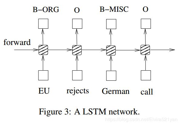
In this paper, we apply Long Short-Term Memory (Hochreiter and Schmidhuber, 1997; Graves et al., 2005) to sequence tagging. Long ShortTerm Memory networks are the same as RNNs, except that the hidden layer updates are replaced by purpose-built memory cells. As a result, they may be better at finding and exploiting long range dependencies in the data. Fig. 2 illustrates a single LSTM memory cell (Graves et al., 2005). The LSTM memory cell is implemented as the following:

在本文中，我们应用了长短期记忆(Hochreiter and Schmidhuber, 1997;Graves et al.， 2005)到序列标记。除了隐藏层更新被专门构建的记忆单元所替代之外，长期和短期内存网络与rnn是相同的。因此，他们可能更善于发现和利用数据中的长期依赖关系。如图2所示，单个LSTM记忆单元(Graves et al.， 2005)。LSTM记忆单元实现如下:

where σ is the logistic sigmoid function, and i, f, o and c are the input gate, forget gate, output gate and cell vectors, all of which are the same size as the hidden vector h. The weight matrix subscripts have the meaning as the name suggests. For example, W_hi is the hidden-input gate matrix, W_xo is the input-output gate matrix etc. The weight matrices from the cell to gate vectors (e.g. W_ci) are diagonal, so element m in each gate vector only receives input from element m of the cell vector.

σ是sigmoid函数.i,f,o和c是和隐藏向量h一样大小的输入门，遗忘门，输出门和单元向量。权重矩阵的下标顾名思义。例如，W_hi是隐藏-输入门矩阵，W_xo是输入-输出门矩阵等。从单元到门向量(如W_ci)的权矩阵是对角线的，所以每个门向量中的元素m只接收来自单元向量的元素m的输入。

Fig. 3 shows a LSTM sequence tagging model which employs aforementioned LSTM memory cells (dashed boxes with rounded corners).

图3所示的LSTM序列标记模型采用了前面提到的LSTM内存单元(虚线框和圆角)。

2.2 Bidirectional LSTM Networks

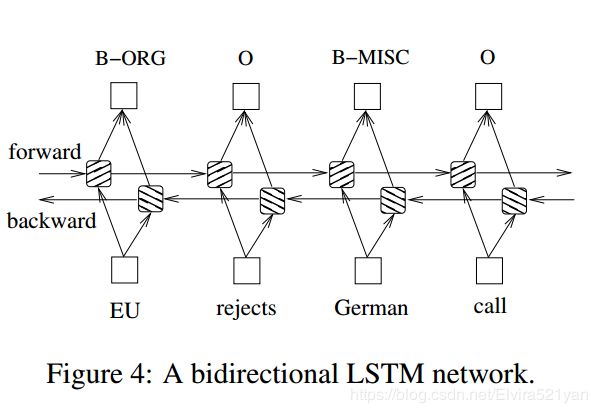
In sequence tagging task, we have access to both past and future input features for a given time, we can thus utilize a bidirectional LSTM network (Figure 4) as proposed in (Graves et al., 2013). In doing so, we can efficiently make use of past features (via forward states) and future features (via backward states) for a specific time frame. We train bidirectional LSTM networks using backpropagation through time (BPTT)(Boden., 2002). The forward and backward passes over the unfolded network over time are carried out in a similar way to regular network forward and backward passes, except that we need to unfold the hidden states for all time steps. We also need a special treatment at the beginning and the end of the data points. In our implementation, we do forward and backward for whole sentences and we only need to reset the hidden states to 0 at the begging of each sentence. We have batch implementation which enables multiple sentences to be processed at the same time .

在序列标记任务中，我们可以在给定的时间内同时获得过去和未来的输入特征，因此我们可以利用双向LSTM网络。在此过程中，我们可以在特定的时间框架内有效地利用过去的特性(通过向前状态)和将来的特性(通过向后状态)。我们使用时间反向传播来训练双向LSTM网络。随着时间的推移，对展开网络的向前和向后传递与常规网络的向前和向后传递类似，只是我们需要对所有时间步骤展开隐藏状态。我们还需要在数据点的开始和结束处进行特殊处理。在我们的实现中，我们对整个句子进行前向和反向操作，我们只需要在每个句子请求时将隐藏状态重置为0。我们有批处理实现，可以同时处理多个句子。

2.3 CRF networks

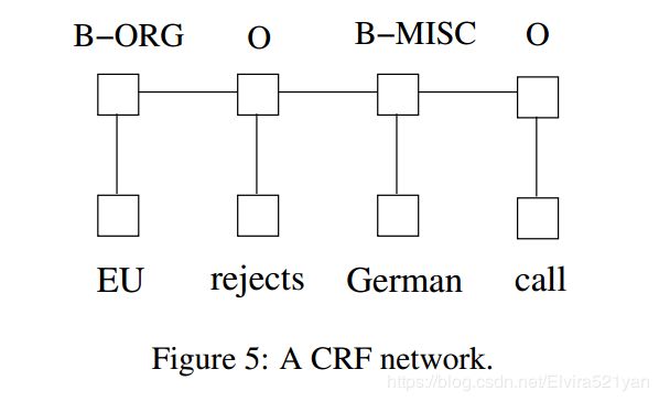
There are two different ways to make use of neighbor tag information in predicting current tags. The first is to predict a distribution of tags for each time step and then use beam-like decoding to find optimal tag sequences. The work of maximum entropy classifier (Ratnaparkhi, 1996) and Maximum entropy Markov models (MEMMs) (McCallum et al., 2000) fall in this category. The second one is to focus on sentence level instead of individual positions, thus leading to Conditional Random Fields (CRF) models (Lafferty et al., 2001) (Fig. 5). Note that the inputs and outputs are directly connected, as opposed to LSTM and bidirectional LSTM networks where memory cells/recurrent components are employed .

在预测当前标签时，有两种可以利用相邻标记信息的不同方法。第一种是预测每一步的标签分布，然后使用波束解码来寻找最优的标签序列。最大熵分类器(Ratnaparkhi, 1996)和最大熵马尔可夫模型(MEMMs) (McCallum et al.， 2000)都属于这一类。 第二种是注重句子层次而不是单个位置，从而引入条件随机字段(CRF)模型(Lafferty et al.， 2001)(图5)。注意，输入和输出是直接连接的，而不是使用记忆细胞/重复成分的LSTM和双向LSTM网络。

2.4 LSTM-CRF networks

We combine a LSTM network and a CRF network to form a LSTM-CRF model, which is shown in Fig. 6. This network can efficiently use past input features via a LSTM layer and sentence level tag information via a CRF layer. A CRF layer is represented by lines which connect consecutive output layers. A CRF layer has a state transition matrix as parameters. With such a layer, we can efficiently use past and future tags to predict the current tag, which is similar to the use of past and future input features via a bidirectional LSTM network. We consider the matrix of scores f${}_{\theta }$($[x]{}_1^T$ ) are output by the network. We drop the input $[x]{}_1^T$for notation simplification. The element [f${}_{\theta }$]_i;t of the matrix is the score output by the network with parameters θ, for the sentence$[x]{}_1^T$ and for the i-th tag, at the t-th word. We introduce a transition score [A]_i;j to model the transition from i-th state to jth for a pair of consecutive time steps. Note that this transition matrix is position independent. We now denote the new parameters for our network as θ~= θ $\bigcup$ {[A]_i;j$\forall$ i,j} The score of a sentence $[x]{}_1^T$ along with a path of tags $[i]{}_1^T$ is then given by the sum of transition scores and network scores:

我们将LSTM网络与CRF网络相结合，形成LSTM-CRF模型，如图6所示。该网络可以通过LSTM层有效地利用过去的输入特征，通过CRF层有效地利用句子级标签信息。CRF层由连接连续输出层的线表示。 CRF层有一个状态转换矩阵作为参数。通过这样的一层，我们可以有效地使用过去和未来的标签来预测当前的标签，这类似于通过双向LSTM网络使用过去和未来的输入特征。我们认为分数的矩阵 f${}_{\theta }$($[x]{}_1^T$ ) 是由网络输出的 。为了简化符号，我们去掉输入$[x]{}_1^T$。 这个矩阵的元素[f${}_{\theta }$]_i;t 是句子$[x]{}_1^T$，第i个标签，第t个词通过带参数 θ的网络计算的分数输出。我们引入一个转换得分[A]_i;j来为一对连续时间步骤从第i状态到第j状态的转换建模。 注意这个转换矩阵是位置无关的 。现在，我们将我们网络的新参数表示为一个句子 $[x]{}_1^T$ 的沿着标签 $[i]{}_1^T$的路径对的分数，这个分数是转移矩阵分数和网络分数之和：

The dynamic programming (Rabiner, 1989) can be used efficiently to compute [A]_i;j and optimal tag sequences for inference. See (Lafferty et al., 2001) for details.

动态规划(Rabiner, 1989)可以有效地计算[A]_i;j 和用于推理的最优标签序列。详见(Lafferty et al.， 2001)

2.5 BI-LSTM-CRF networks

Similar to a LSTM-CRF network, we combine a bidirectional LSTM network and a CRF network to form a BI-LSTM-CRF network (Fig. 7). In addition to the past input features and sentence level tag information used in a LSTM-CRF model, a BILSTM-CRF model can use the future input features. The extra features can boost tagging accuracy as we will show in experiments.

与LSTM-CRF网络相似，我们将双向的LSTM网络与CRF网络相结合，形成一个BI-LSTM-CRF网络(图7)。正如我们将在实验中展示的那样，这些额外的特性可以提高标记的准确性。

3.Training procedure

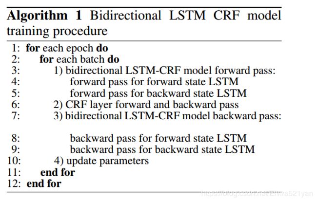
All models used in this paper share a generic SGD forward and backward training procedure. We choose the most complicated model, BI-LSTMCRF, to illustrate the training algorithm as shown in Algorithm 1. In each epoch, we divide the whole training data to batches and process one batch at a time. Each batch contains a list of sentences which is determined by the parameter of batch size. In our experiments, we use batch size of 100 which means to include sentences whose total length is no greater than 100. For each batch, we first run bidirectional LSTM-CRF model forward pass which includes the forward pass for both forward state and backward state of LSTM. As a result, we get the the output score fθ($$[x]{}_1^T$$ ) for all tags at all positions. We then run CRF layer forward and backward pass to compute gradients for network output and state transition edges. After that, we can back propagate the errors from the output to the input, which includes the backward pass for both forward and backward states of LSTM. Finally we update the network parameters which include the state transition matrix [A]_i;j$\forall$ i,j, and the original bidirectional LSTM parameters θ.

本文使用的所有模型都共享一个通用的SGD向前和向后训练过程。我们选择最复杂的模型BI-LSTMCRF来说明训练算法，如算法1所示。在每个阶段，我们将所有的训练数据分成批，一次处理一批。每批包含一个由批大小参数决定的句子列表。在我们的实验中，我们使用批处理大小为100，这意味着包含总长度不大于100的句子。对于每批，我们首先运行双向LSTM- crf模型向前传递，包括LSTM向前状态和向后状态的向前传递。 结果，我们得到了所有位置的所有标签的输出分数。然后，我们向前和向后运行CRF层来计算网络输出和状态转换边缘的梯度。 在这之后，我们可以将误差从输出传播到输入，这包括LSTM向前和向后状态的向后传递 。最后，我们更新网络参数，包括状态转移矩阵[A]_i;j$\forall$ i,j和双向LSTM的的初始参数 θ。

4.Experiments

4.1 Data

We test LSTM, BI-LSTM, CRF, LSTM-CRF, and BI-LSTM-CRF models on three NLP tagging tasks: Penn TreeBank (PTB) POS tagging, CoNLL 2000 chunking, and CoNLL 2003 named entity tagging. Table 1 shows the size of sentences, tokens, and labels for training, validation and test sets respectively.

我们在三个NLP标记任务:Penn TreeBank (PTB) POS标记、CoNLL 2000分块和CoNLL 2003命名实体标记上测试LSTM、BI-LSTM、CRF、LSTM-CRF和BI-LSTM-CRF模型。表1分别显示了用于培训、验证和测试集的句子、令牌和标签的大小。

POS assigns each word with a unique tag that indicates its syntactic role. In chunking, each word is tagged with its phrase type. For example, tag B-NP indicates a word starting a noun phrase. In NER task, each word is tagged with other or one of four entity types: Person, Location, Organization, or Miscellaneous. We use the BIO2 annotation standard for chunking and NER tasks.

POS为每个单词分配一个惟一的标记，该标记指示其语法角色。在分块中，每个单词都有其短语类型标记。例如，标签B-NP表示一个单词开始于一个名词短语。在NER任务中，每个单词都被标记为其他或四种实体类型之一:Person、Location、Organization或杂类。我们使用BIO2注释标准进行分块和NER任务。

4.2 Features

We extract the same types of features for three data sets. The features can be grouped as spelling features and context features. As a result, we have 401K, 76K, and 341K features extracted for POS, chunking and NER data sets respectively. These features are similar to the features extracted from Stanford NER tool (Finkel et al., 2005; Wang and Manning, 2013). Note that we did not use extra data for POS and chunking tasks, with the exception of using Senna embedding (see Section 4.2.3). For NER task, we report performance with spelling and context features, and also incrementally with Senna embedding and Gazetteer features。

我们为三个数据集提取相同类型的特征。这些特征可以分为拼写特征和上下文特征。因此，我们分别提取了POS、分块和NER数据集的401K、76K和341K特征。这些特征与斯坦福NER工具提取的特征相似(Finkel et al.， 2005;Wang and Manning, 2013)。注意，除了使用Senna内嵌之外，对于POS和分块任务，我们没有使用额外的数据(参见4.2.3节)。对于NER任务，我们使用拼写和上下文特征来报告性能，同时也使用Senna嵌入和Gazetteer特征逐步报告性能。

4.2.1 Spelling features

We extract the following features for a given word in addition to the lower case word features.

• whether start with a capital letter

• whether has all capital letters

• whether has all lower case letters

• whether has non initial capital letters

• whether mix with letters and digits

• whether has punctuation

• letter prefixes and suffixes (with window size of 2 to 5)

• whether has apostrophe end (’s)

• letters only, for example, I. B. M. to IBM

• non-letters only, for example, A. T. &T. to …&

• word pattern feature, with capital letters, lower case letters, and digits mapped to ‘A’, ‘a’ and ‘0’ respectively, for example, D56y-3 to A00a-0

• word pattern summarization feature, similar to word pattern feature but with consecutive identical characters removed. For example, D56y-3 to A0a-0

除了小写的单词特征外，我们还提取给定单词的下列特征。

• 是否以大写字母开头
• 是否有所有大写字母
• 是否有所有小写字母
• 是否有非首字母大写
• 是否字母和数字混合
• 是否有标点符号
• 字母前缀和后缀(窗口大小为2到5)
• 是否有撇号结尾(’ s)
• 非字母，例如 A. T. &T. to …&
• 单词模式特征，大写字母、小写字母和数字分别映射到“A”、“A”和“0”，例如，d56 -3到A00a-0
• 词型总结特征，类似于词型特征，但去掉了连续的相同字符。例如，d56 -3到A0a-0

4.2.2 Context features

For word features in three data sets, we use unigram features and bi-grams features. For POS features in CoNLL2000 data set and POS & CHUNK features in CoNLL2003 data set, we use unigram, bi-gram and tri-gram features.

对于三组数据中的词特征，我们分别使用了单字特征和双字特征。对于CoNLL2000数据集中的POS特征和CoNLL2003数据集中的POS & CHUNK特征，我们分别使用了unigram、bi-gram和triple -gram特征 。

4.2.3 Word embedding

It has been shown in (Collobert et al., 2011) that word embedding plays a vital role to improve sequence tagging performance. We downloaded the embedding which has 130K vocabulary size and each word corresponds to a 50-dimensional embedding vector. To use this embedding, we simply replace the one hot encoding word representation with its corresponding 50-dimensional vector.

研究表明，词嵌入对于提高序列标记性能起着至关重要的作用。我们下载了包含130K词汇量的嵌入，每个单词对应一个50维的嵌入向量。为了使用这种嵌入，我们简单地用对应的50维向量替换一个独热编码词表示。

4.2.4 Features connection tricks

We can treat spelling and context features the same as word features. That is, the inputs of networks include both word, spelling and context features. However, we find that direct connections from spelling and context features to outputs accelerate training and they result in very similar tagging accuracy. Fig. 8 illustrates this network in which features have direct connections to outputs of networks. We will report all tagging accuracy using this connection. We note that this usage of features has the same flavor of Maximum Entropy features as used in (Mikolov et al., 2011). The difference is that features collision may occur in (Mikolov et al., 2011) as feature hashing technique has been adopted. Since the output labels in sequence tagging data sets are less than that of language model (usually hundreds of thousands), we can afford to have full connections between features and outputs to avoid potential feature collisions.

我们可以将拼写和上下文特征视为单词特征。也就是说，网络的输入包括单词、拼写和上下文特征。 然而，我们发现从拼写和上下文特征到输出的直接联系加速了训练，并且导致了非常相似的标记准确性。图8所示为特征与网络输出直接连接的网络。我们将使用这个连接报告所有标注的准确性。我们注意到，这种特征的使用与(Mikolov et al.， 2011)中使用的最大熵特征相同。不同之处在于(Mikolov et al.， 2011)由于采用了特征哈希技术，可能会发生特征碰撞(feature collision)。由于序列标签数据集的输出标签比语言模型的输出标签少(通常是几十万)，因此我们可以在特征和输出之间建立完整的连接，避免潜在的特征冲突。

4.3 Results

We train LSTM, BI-LSTM, CRF, LSTM-CRF and BI-LSTM-CRF models for each data set. We have two ways to initialize word embedding: Random and Senna. We randomly initialize the word embedding vectors in the first category, and use Senna word embedding in the second category. For each category, we use identical feature sets, thus different results are solely due to different networks. We train models using training data and monitor performance on validation data. As chunking data do not have a validation data set, we use part of training data for validation purpose .

我们为每个数据集训练LSTM、BI-LSTM、CRF、LSTM-CRF和BI-LSTM-CRF模型。我们有两种方法初始化词嵌入： Random 和 Senna.我们在第一类中随机初始化词嵌入向量，在第二类中使用Senna词嵌入。对于每个类别，我们使用相同的特征集，因此不同的结果完全是由于不同的网络。我们使用训练数据对模型进行训练，并用验证集对模型验证。由于分块数据没有验证数据集，因此我们使用部分训练数据进行验证。

We use a learning rate of 0.1 to train models. We set hidden layer size to 300 and found that model performance is not sensitive to hidden layer sizes. The training for three tasks require less than 10 epochs to converge and it in general takes less than a few hours. We report models’ performance on test datasets in Table 2, which also lists the best results in (Collobert et al., 2011), denoted as Conv-CRF. The POS task is evaluated by computing per-word accuracy, while the chunk and NER tasks are evaluated by computing F1 scores over chunks.

我们使用0.1的学习率来训练模型。我们将隐层大小设置为300，发现模型性能对隐层大小并不敏感。三种任务的训练需要不到10个阶段的时间来收敛，通常需要不到几个小时。我们在表2中报告了模型在测试数据集上的性能，表2也列出了(Collobert et al.， 2011)中的最佳结果，记为Conv-CRF。POS任务通过计算每个单词的准确性进行评估，而chunk和NER任务通过计算chunk上的F1分数进行评估 。

4.3.1 Comparison with Cov-CRF networks

We have three baselines: LSTM, BI-LSTM and CRF. LSTM is the weakest baseline for all three data sets. The BI-LSTM performs close to CRF on POS and chunking datasets, but is worse than CRF on NER data set. The CRF forms strong baselines in our experiments. For random category, CRF models outperform Conv-CRF models for all three data sets. For Senna category, CRFs outperform Conv-CRF for POS task, while underperform for chunking and NER task. LSTM-CRF models outperform CRF models for all data sets in both random and Senna categories. This shows the effectiveness of the forward state LSTM component in modeling sequence data. The BI-LSTMCRF models further improve LSTM-CRF models and they lead to the best tagging performance for all cases except for POS data at random category, in which LSTM-CRF model is the winner. The numbers in parentheses for CoNLL 2003 under Senna categories are generated with Gazetteer features.

我们有三个基线:LSTM、BI-LSTM和CRF。LSTM是三个数据集最弱的基线。BI-LSTM在POS和分块数据集上的性能接近CRF，但在NER数据集上的性能较差。在我们的实验中，CRF形成了较强的基线。对于随机类别，CRF模型在三个数据集上都优于Conv-CRF模型。在Senna类别中，crf在POS任务上优于Conv-CRF，而在分块和NER任务上表现不佳。LSTM-CRF模型在随机和Senna类别的所有数据集上都优于CRF模型。这说明了正向状态LSTM组件在序列数据建模中的有效性。BI-LSTMCRF模型进一步改进了LSTM-CRF模型，使得LSTM-CRF模型在所有情况下的标签性能都是最好的，除了随机分类的POS数据，其中LSTM-CRF模型是赢家。在Senna类别下，CoNLL 2003括号中的数字是根据Gazetteer功能生成的。

It is interesting that our best model BI-LSTMCRF has less dependence on Senna word embedding compared to Conv-CRF model. For example, the tagging difference between BI-LSTMCRF model for random and Senna categories are 0.12%, 0.33%, and 4.57% for POS, chunking and NER data sets respectively. In contrast, the ConvCRF model heavily relies on Senna embedding to get good tagging accuracy. It has the tagging difference of 0.92%, 3.99% and 7.20% between random and Senna category for POS, chunking and NER data sets respectively.

有趣的是，与Conv-CRF模型相比，我们的最佳模型BI-LSTMCRF对Senna词嵌入的依赖更小。例如，对于随机类别和Senna类别，BI-LSTMCRF模型的标记差异分别为0.12%、0.33%和4.57%，对于POS、chunking和NER数据集的标记差异分别为0.12%、0.33%和4.57%。而ConvCRF模型在很大程度上依赖于Senna的嵌入来获得良好的标注精度。对于POS、分块和NER数据集，random和Senna类别的标签差异分别为0.92%、3.99%和7.20%。

4.3.2 Model robustness

To estimate the robustness of models with respect to engineered features (spelling and context features), we train LSTM, BI-LSTM, CRF, LSTMCRF, and BI-LSTM-CRF models with word features only (spelling and context features removed). Table 3 shows tagging performance of proposed models for POS, chunking, and NER data sets using Senna word embedding. The numbers in parentheses indicate the performance degradation compared to the same models but using spelling and context features. CRF models’ performance is significantly degraded with the removal of spelling and context features. This reveals the fact that CRF models heavily rely on engineered features to obtain good performance. On the other hand, LSTM based models, especially BI-LSTM and BI-LSTM-CRF models are more robust and they are less affected by the removal of engineering features. For all three tasks, BI-LSTM-CRF models result in the highest tagging accuracy. For example, It achieves the F1 score of 94.40 for CoNLL2000 chunking, with slight degradation (0.06) compared to the same model but using spelling and context features.

为了评估模型相对于工程特性(拼写和上下文特性)的鲁棒性，我们对LSTM、BI-LSTM、CRF、LSTMCRF和BI-LSTM-CRF模型进行了培训，这些模型只包含单词特性(删除了拼写和上下文特性)。表3显示了使用Senna词嵌入的POS、分块和NER数据集模型的标记性能。括号中的数字表明，与使用拼写和上下文特性的相同模型相比，性能有所下降。CRF模型的性能随着拼写和上下文特征的去除而显著下降。这揭示了CRF模型严重依赖工程特性来获得良好性能的事实。另一方面，基于LSTM的模型，尤其是BI-LSTM和BI-LSTM- crf模型更健壮，不受工程特性的影响。对于这三个任务，BI-LSTM-CRF模型的标记精度最高。例如CoNLL2000 chunking的F1得分为94.40，与相同的模型相比，在使用拼写和上下文特征的情况下，有轻微的下降(0.06)。

4.3.3 Comparison with existing systems

For POS data set, we achieved state of the art tagging accuracy with or without the use of extra data resource. POS data set has been extensively tested and the past improvement can be realized in Table 4. Our test accuracy is 97.55% which is significantly better than others in the confidence level of 95%. In addition, our BI-LSTM-CRF model already reaches a good accuracy without the use of the Senna embedding.

对于POS数据集，无论是否使用额外的数据资源，我们都实现了最先进的标注精度。POS数据集经过了广泛的测试，过去的改进如表4所示。我们的测试准确率为97.55%，在95%的置信度水平上显著优于其他测试。此外，我们的BI-LSTM-CRF模型在不使用Senna嵌入的情况下已经达到了较好的精度。

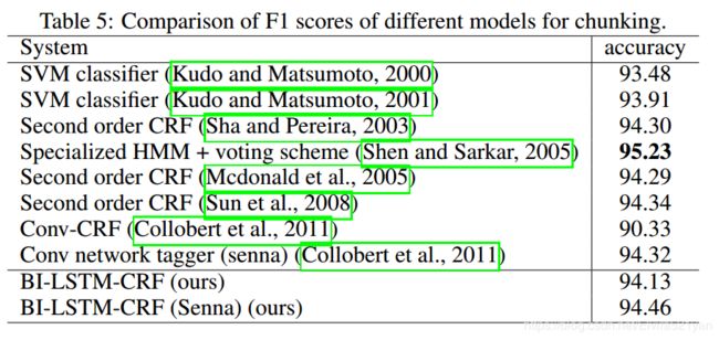
All chunking systems performance is shown in table 5. Kudo et al. won the CoNLL 2000 challenge with a F1 score of 93.48%. Their approach was a SVM based classifier. They later improved the results up to 93.91%. Recent work include the CRF based models (Sha and Pereira, 2003; Mcdonald et al., 2005; Sun et al., 2008). More recent is (Shen and Sarkar, 2005) which obtained 95.23% accuracy with a voting classifier scheme, where each classifier is trained on different tag representations (IOB, IOE, etc.). Our model outperforms all reported systems except (Shen and Sarkar, 2005).

所有分块系统的性能如表5所示。Kudo等人以93.48%的F1成绩赢得了CoNLL 2000挑战赛。他们的方法是基于SVM的分类器。他们后来将结果提高到了93.91%。最近的工作包括基于CRF的模型(Sha和Pereira, 2003;Mcdonald et al.， 2005;Sun等人，2008)。最近的是(Shen and Sarkar, 2005)，他们使用投票分类器方案获得了95.23%的准确率，每个分类器在不同的标签表示(IOB, IOE等)上进行训练。除了(Shen and Sarkar, 2005)，我们的模型优于所有报告的系统。

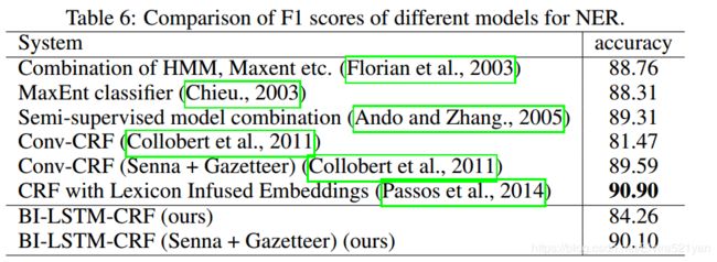
The performance of all systems for NER is shown in table 6. (Florian et al., 2003) presented the best system at the NER CoNLL 2003 challenge, with 88.76% F1 score. They used a combination of various machine-learning classifiers. The second best performer of CoNLL 2003 (Chieu., 2003) was 88.31% F1, also with the help of an external gazetteer. Later, (Ando and Zhang., 2005) reached 89.31% F1 with a semi-supervised approach. The best F1 score of 90.90% was reported in (Passos et al., 2014) which employed a new form of learning word embeddings that can leverage information from relevant lexicons to improve the representations. Our model can achieve the best F1 score of 90.10 with both Senna embedding and gazetteer features. It has a lower F1 score than (Passos et al., 2014) , which may be due to the fact that different word embeddings were employed. With the same Senna embedding, BI-LSTM-CRF slightly outperforms Conv-CRF (90.10% vs. 89.59%). However, BI-LSTM-CRF significantly outperforms Conv-CRF (84.26% vs. 81.47%) if random embedding is used.

NER的所有系统的性能如表6所示。(Florian et al.， 2003)在2003年NER CoNLL挑战赛中以88.76%的F1成绩获得最佳系统。他们使用了各种机器学习分类器的组合。2003年CoNLL (Chieu., 2003)第二名最好的性能为则为88.31% F1，也是在外部gazetteer的协助下。后来， (Ando and Zhang., 2005) ，在半监督方法下，达到89.31% F1。F1得分最高的是(Passos et al.， 2014)达到了90.90%，采用了一种新的学习嵌入词的形式——可以利用相关词汇的信息来改善表征。我们的模型结合了Senna嵌入和gazetteer的特征，可以获得90.10的F1最好成绩。F1得分低于(Passos et al.， 2014)，这可能是因为使用了不同的单词嵌入。在相同的Senna嵌入情况下，BI-LSTM-CRF的表现略优于Conv-CRF (90.10% vs. 89.59%)。然而，如果使用随机嵌入，BI-LSTM-CRF显著优于Conv-CRF (84.26% vs. 81.47%)。

5.Discussions

Our work is close to the work of (Collobert et al., 2011) as both of them utilized deep neural networks for sequence tagging. While their work used convolutional neural networks, ours used bidirectional LSTM networks.

我们的工作与(Collobert et al.， 2011)的工作非常接近，因为都使用深层神经网络进行序列标记。他们的工作使用卷积神经网络，而我们的工作使用双向LSTM网络。

Our work is also close to the work of (Hammerton, 2003; Yao et al., 2014) as all of them employed LSTM network for tagging. The performance in (Hammerton, 2003) was not impressive. The work in (Yao et al., 2014) did not make use of bidirectional LSTM and CRF layers and thus the tagging accuracy may be suffered.

我们的工作也与(Hammerton, 2003;Yao等人，2014)非常接近，因为都使用LSTM网络进行标记。(Hammerton, 2003)的表现并不令人印象深刻。(Yao et al.， 2014)的工作没有使用双向LSTM和CRF层，可能会影响标签的准确性 。

Finally, our work is related to the work of (Wang and Manning, 2013) which concluded that non-linear architecture offers no benefits in a highdimensional discrete feature space. We showed that with the bi-directional LSTM CRF model, we consistently obtained better tagging accuracy than a single CRF model with identical feature sets.

最后，我们的工作与(Wang and Manning, 2013)的工作有关，他们得出结论，非线性建筑在高维离散特征空间中没有优势。结果表明，在双向LSTM CRF模型中，我们的标记精度始终优于单一特征集相同的CRF模型。

6.Conclusions

In this paper, we systematically compared the performance of LSTM networks based models for sequence tagging. We presented the first work of applying a BI-LSTM-CRF model to NLP benchmark sequence tagging data. Our model can produce state of the art (or close to) accuracy on POS, chunking and NER data sets. In addition, our model is robust and it has less dependence on word embedding as compared to the observation in (Collobert et al., 2011). It can achieve accurate tagging accuracy without resorting to word embedding.

本文系统地比较了基于LSTM网络的序列标记模型的性能。我们提出了将BI-LSTM-CRF模型应用于NLP基准序列标记数据的第一个工作。我们的模型可以在POS、分块和NER数据集上产生最先进(或接近)的准确性。此外，我们的模型是稳健的，与(Collobert et al.， 2011)中的观察相比，它对嵌入词的依赖更少。它不需要嵌入词就可以实现精确的标注精度。

（注：若有错误希望大家指出！）