吴恩达Coursera深度学习课程 DeepLearning.ai 编程作业——Regularization（2-1.2）

如果数据集没有很大，同时在训练集上又拟合得很好，但是在测试集的效果却不是很好，这时候就要使用正则化来使得其拟合能力不会那么强。

import numpy as np
import sklearn
import matplotlib.pyplot as plt
import sklearn.datasets
from reg_utils import load_2D_dataset,compute_cost,forward_propagation,predict,predict_dec,relu,sigmoid
from reg_utils import initialize_parameters,backward_propagation,update_parameters,plot_decision_boundary
import scipy.io

plt.rcParams["figure.figsize"]=(7,4)  #the figure size，which wight is 7，while height is 4
plt.rcParams["image.interpolation"]="nearest"  #
plt.rcParams["image.cmap"]="gray"

train_x,train_y,test_x,test_x,test_y=load_2D_dataset()

import numpy as np
import matplotlib.pyplot as plt
import h5py
import sklearn
import sklearn.datasets
import sklearn.linear_model
import scipy.io

####reg_utils.py#####  以下是reg_utils.py 文件的内容

def sigmoid(x):
    s = 1/(1+np.exp(-x))
    return s

def relu(x):
    s = np.maximum(0,x)
    return s

def load_planar_dataset(seed):
    
    np.random.seed(seed)    
    m = 400 # number of examples
    N = int(m/2) # number of points per class
    D = 2 # dimensionality
    X = np.zeros((m,D)) # data matrix where each row is a single example
    Y = np.zeros((m,1), dtype='uint8') # labels vector (0 for red, 1 for blue)
    a = 4 # maximum ray of the flower
    for j in range(2):
        ix = range(N*j,N*(j+1))
        t = np.linspace(j*3.12,(j+1)*3.12,N) + np.random.randn(N)*0.2 # theta
        r = a*np.sin(4*t) + np.random.randn(N)*0.2 # radius
        X[ix] = np.c_[r*np.sin(t), r*np.cos(t)]
        Y[ix] = j       
    X = X.T
    Y = Y.T

    return X, Y

def initialize_parameters(layer_dims):
    """
    Arguments:
    layer_dims -- python array (list) containing the dimensions of each layer in our network    
    Returns:
    parameters -- python dictionary containing your parameters "W1", "b1", ..., "WL", "bL":
                    W1 -- weight matrix of shape (layer_dims[l], layer_dims[l-1])
                    b1 -- bias vector of shape (layer_dims[l], 1)
                    Wl -- weight matrix of shape (layer_dims[l-1], layer_dims[l])
                    bl -- bias vector of shape (1, layer_dims[l])                    
    Tips:
    - For example: the layer_dims for the "Planar Data classification model" would have been [2,2,1]. 
    This means W1's shape was (2,2), b1 was (1,2), W2 was (2,1) and b2 was (1,1). Now you have to generalize it!
    - In the for loop, use parameters['W' + str(l)] to access Wl, where l is the iterative integer.
    """   
    np.random.seed(3)
    parameters = {}
    L = len(layer_dims) # number of layers in the network

    for l in range(1, L):
        parameters['W' + str(l)] = np.random.randn(layer_dims[l], layer_dims[l-1]) / np.sqrt(layer_dims[l-1])
        parameters['b' + str(l)] = np.zeros((layer_dims[l], 1))
        
        assert(parameters['W' + str(l)].shape == layer_dims[l], layer_dims[l-1])
        assert(parameters['W' + str(l)].shape == layer_dims[l], 1)        
    return parameters

def forward_propagation(X, parameters):
    """
    Implements the forward propagation (and computes the loss) presented in Figure 2.
    
    Arguments:
    X -- input dataset, of shape (input size, number of examples)
    parameters -- python dictionary containing your parameters "W1", "b1", "W2", "b2", "W3", "b3":
                    W1 -- weight matrix of shape ()
                    b1 -- bias vector of shape ()
                    W2 -- weight matrix of shape ()
                    b2 -- bias vector of shape ()
                    W3 -- weight matrix of shape ()
                    b3 -- bias vector of shape ()
     Returns:
    loss -- the loss function (vanilla logistic loss)
    """        
    # retrieve parameters
    W1 = parameters["W1"]
    b1 = parameters["b1"]
    W2 = parameters["W2"]
    b2 = parameters["b2"]
    W3 = parameters["W3"]
    b3 = parameters["b3"]    
    # LINEAR -> RELU -> LINEAR -> RELU -> LINEAR -> SIGMOID
    Z1 = np.dot(W1, X) + b1
    A1 = relu(Z1)
    Z2 = np.dot(W2, A1) + b2
    A2 = relu(Z2)
    Z3 = np.dot(W3, A2) + b3
    A3 = sigmoid(Z3)
    
    cache = (Z1, A1, W1, b1, Z2, A2, W2, b2, Z3, A3, W3, b3)
    
    return A3, cache

def backward_propagation(X, Y, cache):
    """
    Implement the backward propagation presented in figure 2.    
    Arguments:
    X -- input dataset, of shape (input size, number of examples)
    Y -- true "label" vector (containing 0 if cat, 1 if non-cat)
    cache -- cache output from forward_propagation()
    
    Returns:
    gradients -- A dictionary with the gradients with respect to each parameter, activation and pre-activation variables
    """
    m = X.shape[1]
    (Z1, A1, W1, b1, Z2, A2, W2, b2, Z3, A3, W3, b3) = cache
    
    dZ3 = A3 - Y
    dW3 = 1./m * np.dot(dZ3, A2.T)
    db3 = 1./m * np.sum(dZ3, axis=1, keepdims = True)
    
    dA2 = np.dot(W3.T, dZ3)
    dZ2 = np.multiply(dA2, np.int64(A2 > 0))
    dW2 = 1./m * np.dot(dZ2, A1.T)
    db2 = 1./m * np.sum(dZ2, axis=1, keepdims = True)
    
    dA1 = np.dot(W2.T, dZ2)
    dZ1 = np.multiply(dA1, np.int64(A1 > 0))
    dW1 = 1./m * np.dot(dZ1, X.T)
    db1 = 1./m * np.sum(dZ1, axis=1, keepdims = True)
    
    gradients = {"dZ3": dZ3, "dW3": dW3, "db3": db3,
                 "dA2": dA2, "dZ2": dZ2, "dW2": dW2, "db2": db2,
                 "dA1": dA1, "dZ1": dZ1, "dW1": dW1, "db1": db1}
    
    return gradients

def update_parameters(parameters, grads, learning_rate):
    """
    Update parameters using gradient descent    
    Arguments:
    parameters -- python dictionary containing your parameters:
                    parameters['W' + str(i)] = Wi
                    parameters['b' + str(i)] = bi
    grads -- python dictionary containing your gradients for each parameters:
                    grads['dW' + str(i)] = dWi
                    grads['db' + str(i)] = dbi
    learning_rate -- the learning rate, scalar.    
    Returns:
    parameters -- python dictionary containing your updated parameters 
    """
    n = len(parameters) // 2 # number of layers in the neural networks

    # Update rule for each parameter
    for k in range(n):
        parameters["W" + str(k+1)] = parameters["W" + str(k+1)] - learning_rate * grads["dW" + str(k+1)]
        parameters["b" + str(k+1)] = parameters["b" + str(k+1)] - learning_rate * grads["db" + str(k+1)]
        
    return parameters

def predict(X, y, parameters):
    """
    This function is used to predict the results of a  n-layer neural network.    
    Arguments:
    X -- data set of examples you would like to label
    parameters -- parameters of the trained model    
    Returns:
    p -- predictions for the given dataset X
    """    
    m = X.shape[1]
    p = np.zeros((1,m), dtype = np.int)
    
    # Forward propagation
    a3, caches = forward_propagation(X, parameters)    
    # convert probas to 0/1 predictions
    for i in range(0, a3.shape[1]):
        if a3[0,i] > 0.5:
            p[0,i] = 1
        else:
            p[0,i] = 0
    # print results

    #print ("predictions: " + str(p[0,:]))
    #print ("true labels: " + str(y[0,:]))
    print("Accuracy: "  + str(np.mean((p[0,:] == y[0,:]))))
    
    return p
def compute_cost(a3, Y):
    """
    Implement the cost function    
    Arguments:
    a3 -- post-activation, output of forward propagation
    Y -- "true" labels vector, same shape as a3    
    Returns:
    cost - value of the cost function
    """
    m = Y.shape[1] 
    logprobs = np.multiply(-np.log(a3),Y) + np.multiply(-np.log(1 - a3), 1 - Y)
    cost = 1./m * np.nansum(logprobs)
   
    return cost

def load_dataset():
    train_dataset = h5py.File('datasets/train_catvnoncat.h5', "r")
    train_set_x_orig = np.array(train_dataset["train_set_x"][:]) # your train set features
    train_set_y_orig = np.array(train_dataset["train_set_y"][:]) # your train set labels

    test_dataset = h5py.File('datasets/test_catvnoncat.h5', "r")
    test_set_x_orig = np.array(test_dataset["test_set_x"][:]) # your test set features
    test_set_y_orig = np.array(test_dataset["test_set_y"][:]) # your test set labels

    classes = np.array(test_dataset["list_classes"][:]) # the list of classes
    
    train_set_y = train_set_y_orig.reshape((1, train_set_y_orig.shape[0]))
    test_set_y = test_set_y_orig.reshape((1, test_set_y_orig.shape[0]))
    
    train_set_x_orig = train_set_x_orig.reshape(train_set_x_orig.shape[0], -1).T
    test_set_x_orig = test_set_x_orig.reshape(test_set_x_orig.shape[0], -1).T
    
    train_set_x = train_set_x_orig/255
    test_set_x = test_set_x_orig/255

    return train_set_x, train_set_y, test_set_x, test_set_y, classes


def predict_dec(parameters, X):
    """
    Used for plotting decision boundary.  
    Arguments:
    parameters -- python dictionary containing your parameters 
    X -- input data of size (m, K) 
    Returns
    predictions -- vector of predictions of our model (red: 0 / blue: 1)
    """   
    # Predict using forward propagation and a classification threshold of 0.5
    a3, cache = forward_propagation(X, parameters)
    predictions = (a3>0.5)
    return predictions

def load_planar_dataset(randomness, seed):  
    np.random.seed(seed)  
    m = 50
    N = int(m/2) # number of points per class
    D = 2 # dimensionality
    X = np.zeros((m,D)) # data matrix where each row is a single example
    Y = np.zeros((m,1), dtype='uint8') # labels vector (0 for red, 1 for blue)
    a = 2 # maximum ray of the flower

    for j in range(2):      
        ix = range(N*j,N*(j+1))
        if j == 0:
            t = np.linspace(j, 4*3.1415*(j+1),N) #+ np.random.randn(N)*randomness # theta
            r = 0.3*np.square(t) + np.random.randn(N)*randomness # radius
        if j == 1:
            t = np.linspace(j, 2*3.1415*(j+1),N) #+ np.random.randn(N)*randomness # theta
            r = 0.2*np.square(t) + np.random.randn(N)*randomness # radius
            
        X[ix] = np.c_[r*np.cos(t), r*np.sin(t)]
        Y[ix] = j
        
    X = X.T
    Y = Y.T

    return X, Y

def plot_decision_boundary(model, X, y):
    # Set min and max values and give it some padding
    x_min, x_max = X[0, :].min() - 1, X[0, :].max() + 1
    y_min, y_max = X[1, :].min() - 1, X[1, :].max() + 1
    h = 0.01
    # Generate a grid of points with distance h between them
    xx, yy = np.meshgrid(np.arange(x_min, x_max, h), np.arange(y_min, y_max, h))
    # Predict the function value for the whole grid
    print ("the input shape"+str(np.c_[xx.ravel(),yy.ravel()].shape))
    Z = model(np.c_[xx.ravel(), yy.ravel()])
    Z = Z.reshape(xx.shape)
    # Plot the contour and training examples
    plt.contourf(xx, yy, Z, cmap=plt.cm.Spectral)
    plt.ylabel('x2')
    plt.xlabel('x1')
    plt.scatter(X[0, :], X[1, :], c=y, cmap=plt.cm.Spectral)
    plt.show()
    
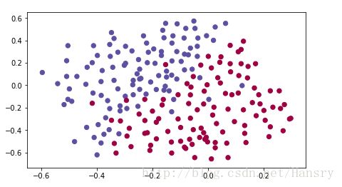
def load_2D_dataset():
    data = scipy.io.loadmat('/home/hansry/python/DL/2-1/week1_Regularization/datasets/data.mat.mat')
    train_X = data['X'].T
    train_Y = data['y'].T
    test_X = data['Xval'].T
    test_Y = data['yval'].T    
    plt.scatter(train_X[0, :], train_X[1, :], c=train_Y, s=40, cmap=plt.cm.Spectral);
    plt.show()
    return train_X, train_Y, test_X, test_Y

1. Non-regularization model

---

def model(X,Y,learning_rate=0.3,num_iterations=30000,print_cost=True,lambd=0,keep_prob=1):
    grads={}
    costs=[]
    m=X.shape[1]
    layers_dims=[X.shape[0],20,3,1]
    
    #Initialize=initialize_parameters(layers_dims)
    parameters=initialize_parameters(layers_dims)     
    for i in range(0, num_iterations)：        
        # Forward propagation: LINEAR -> RELU -> LINEAR -> RELU -> LINEAR -> SIGMOID.
        
        if keep_prob == 1:    
            a3, cache = forward_propagation(X, parameters)
        elif keep_prob < 1:   #当keep_prob<1时，使用drop_out,其中keep_prob between 0 and 1
            a3, cache,cache_Dl = forward_propagation_with_dropout(X, parameters, keep_prob)        
            
        # Cost function
        if lambd == 0:   
            cost = compute_cost(a3, Y)
        else:   #如果lambd不等于0，那么使用regulrization
            cost = compute_cost_with_regularization(a3, Y, parameters, lambd)

        # Backward propagation.
        assert(lambd==0 or keep_prob==1)    # it is possible to use both L2 regularization and dropout, 
                                            # but this assignment will only explore one at a time
        if lambd == 0 and keep_prob == 1:
            grads = backward_propagation(X, Y, cache)
        elif lambd != 0:
            grads = backward_propagation_with_regularization(X, Y, cache, lambd)
        elif keep_prob < 1:
            grads = backward_propogation_with_dropout(X,Y,cache,cache_Dl,keep_prob)
            
        # Update parameters.
        parameters = update_parameters(parameters, grads, learning_rate)
        
        # Print the loss every 10000 iterations
        if print_cost and i % 10000 == 0:
            print("Cost after iteration {}: {}".format(i, cost))
        if print_cost and i % 1000 == 0:
            costs.append(cost)
    
    # plot the cost
    plt.plot(costs)
    plt.ylabel('cost')
    plt.xlabel('iterations (x1,000)')
    plt.title("Learning rate =" + str(learning_rate))
    plt.show()
    
    return parameters

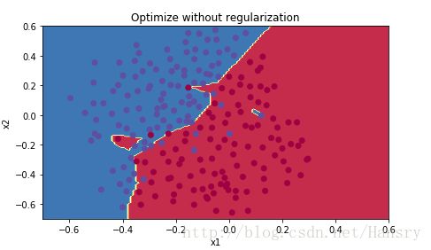
parameters=model(train_x,train_y,learning_rate=0.3,num_iterations=30000,print_cost=True,lambd=0,keep_prob=1)
print train_x.shape
print("On the train do not use regularization and dropout")  
train_prediction=predict(train_x,train_y,parameters)
print ("On the test do not use regularization and dropout")
test_prediction=predict(test_x,test_y,parameters)


plt.title("Optimize without regularization")
axes=plt.gca()
axes.set_xlim([-0.7,0.6])
axes.set_ylim([-0.7,0.6])
plot_decision_boundary(lambda x: predict_dec(parameters,x.T),train_x,train_y)

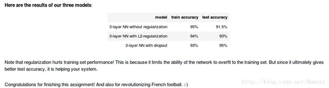
Expected Output：

Cost after iteration 0: 0.655741252348
Cost after iteration 10000: 0.163299875257
Cost after iteration 20000: 0.138516424233

On the train do not use regularization and dropout
Accuracy: 0.947867298578
On the test do not use regularization and dropout
Accuracy: 0.915

2. L2 Regularization

---

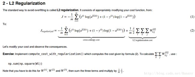
def compute_cost_with_regularization(A3,Y,parameters,lamda): #将L2正则化添加到公式中
    m=Y.shape[1]
    L=len(parameters)//2
    regularization_sum=0.0
    for l in range(L):
        regularization_sum += np.sum(np.square(parameters["W"+str(l+1)]))
    
    regularization_cost=(lamda/(2.0*m))*regularization_sum
    cost_entropy=compute_cost(A3,Y)
    cost=cost_entropy+regularization_cost
    return cost

'''
a3, Y_assess, parameters=compute_cost_with_regularization_test_case()
cost=compute_cost_with_regularization(a3,Y_assess,parameters,lamda=0.1)
print cost
'''
    
def backward_propagation_with_regularization(X,Y,caches,lamda):   #这个函数对于多层神经网络均适用
    L=len(caches)//4
    cache={}
    m=X.shape[1]
    grads={}
    for i in range(0,L):
        cache["Z"+str(i+1)]=caches[i*4]
        cache["A"+str(i+1)]=caches[i*4+1]
        cache["W"+str(i+1)]=caches[i*4+2]
        cache["b"+str(i+1)]=caches[i*4+3]
    grads["dZ"+str(L)]=cache["A"+str(L)]-Y
    grads["dW"+str(L)]=(1.0/m)*np.dot(grads["dZ"+str(L)],cache["A"+str(L-1)].T)+np.float(lamda/m)*cache["W"+str(L)]
    grads["db"+str(L)]=(1.0/m)*np.sum(grads["dZ"+str(L)],axis=1,keepdims=True)
    grads["dA"+str(L-1)]=np.dot(cache["W"+str(L)].T,grads["dZ"+str(L)])
    for l in reversed(range(1,L)):
        if l > 1:
            grads["dZ"+str(l)]=np.multiply(grads["dA"+str(l)],np.int64(cache["A"+str(l)]>0))
 #       grads["dW"+str(l)]=cache["A"+str(L)]-Y
            grads["dW"+str(l)]=(1.0/m)*np.dot(grads["dZ"+str(l)],cache["A"+str(l-1)].T)+np.float(lamda/m)*cache["W"+str(l)]
            grads["db"+str(l)]=(1.0/m)*np.sum(grads["dZ"+str(l)],axis=1,keepdims=True)
            grads["dA"+str(l-1)]=np.dot(cache["W"+str(l)].T,grads["dZ"+str(l)])
        elif l==1:
            grads["dZ"+str(1)]=np.multiply(grads["dA"+str(1)],np.int64(cache["A"+str(1)]>0))
            grads["dW"+str(1)]=(1.0/m)*np.dot(grads["dZ"+str(1)],X.T)+np.float(lamda/m)*cache["W"+str(1)]
            grads["db"+str(1)]=(1.0/m)*np.sum(grads["dZ"+str(1)],axis=1,keepdims=True)
    return grads


#test the correctness of backward_propagation 
"""
X_assess,Y_assess,cache=backward_propagation_with_regularization_test_case()
grads=backward_propagation_with_regularization(X_assess,Y_assess,cache,lamda=0.7)
print ("dW1 :"+str(grads["dW1"]))
print ("dW2 :"+str(grads["dW2"]))
print ("dW3 :"+str(grads["dW3"]))

"""

#remerber to recover the codes below
parameters_with_regularization=model(train_x,train_y,learning_rate=0.3,num_iterations=30000,print_cost=True,lambd=0.7,keep_prob=1)
print("On the train with regularization")
train_prediction_regularization=predict(train_x,train_y,parameters_with_regularization)

print ("On the test with regularization")
test_prediction_regularization=predict(test_x,test_y,parameters_with_regularization)

plt.title("Optimize with regularization")
axes=plt.gca()
axes.set_xlim([-0.7,0.6])
axes.set_ylim([-0.7,0.6])
plot_decision_boundary(lambda x: predict_dec(parameters_with_regularization,x.T),train_x,train_y)

Expected output：

Cost after iteration 0: 0.697448449313
Cost after iteration 10000: 0.268491887328
Cost after iteration 20000: 0.268091633713

On the train with regularization
Accuracy: 0.938388625592
On the test with regularization
Accuracy: 0.93

3.forward and backward propagation with dropout

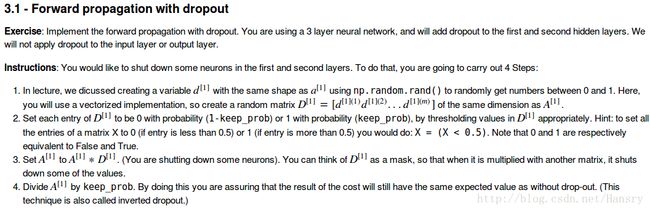
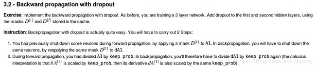
def forward_propagation_with_dropout(X,parameters,keep_prob=0.5):
    cache=[] #list
    cache_D={}  #dictionary
    L=len(parameters)//2
    W1=parameters["W1"]
    b1=parameters["b1"]
    Z1=np.dot(W1,X)+b1
    A1=relu(Z1)
    cache=[Z1,A1,W1,b1]
    np.random.seed(1)
    for l in range(1,L):
        cache_D["D"+str(l)]=np.random.rand(cache[4*(l-1)+1].shape[0],cache[4*(l-1)+1].shape[1])   #randn(A1.shape[0],A1.shape[]1)
        cache_D["D"+str(l)]=np.where(cache_D["D"+str(l)]<=keep_prob,1,0)    # D1
        cache[4*(l-1)+1]=np.multiply(cache[4*(l-1)+1],cache_D["D"+str(l)])  # A1,eliminate some neure randomly
        cache[4*(l-1)+1]=cache[4*(l-1)+1]/keep_prob
        cache_4l=np.dot(parameters["W"+str(l+1)],cache[4*(l-1)+1])+parameters["b"+str(l+1)]  # cache[4*l]  Z2
        cache.append(cache_4l)
        if l==(L-1):
            cache_4l_plus1=sigmoid(cache[4*l])  #A2,A3,...
        elif l0)) #dZ2(3,5)
        if l>1:
            grads["dW"+str(l)]=(1.0/m)*np.dot(grads["dZ"+str(l)],cache[4*(l-2)+1].T)   # dW2(3,2)=dZ2(3,5)*A1(2,5).T
        elif l==1:
            grads["dW"+str(l)]=(1.0/m)*np.dot(grads["dZ"+str(l)],X.T)
        grads["db"+str(l)]=(1.0/m)*np.sum(grads["dZ"+str(l)],axis=1,keepdims=True)
        grads["dA"+str(l-1)]=np.dot(cache[4*(l-1)+2].T,grads["dZ"+str(l)])
    return grads

parameters_with_dropout=model(train_x,train_y,keep_prob=0.86,learning_rate=0.3)
print ("On the train set with dropout:")
predictions_train = predict(train_x, train_y, parameters_with_dropout)
print ("On the test set with dropout:")
predictions_test = predict(test_x, test_y, parameters_with_dropout)          

plt.title("the cost curve with ")
axes=plt.gca()
axes.set_xlim([-0.7,0.6])
axes.set_ylim([-0.7,0.6])
plot_decision_boundary(lambda x:predict_dec(parameters_with_dropout,x.T),train_x,train_y）

Expected output：

Cost after iteration 0: 0.654391240515
reg_utils.py:238: RuntimeWarning: divide by zero encountered in log
  logprobs = np.multiply(-np.log(a3),Y) + np.multiply(-np.log(1 - a3), 1 - Y)
reg_utils.py:238: RuntimeWarning: invalid value encountered in multiply
  logprobs = np.multiply(-np.log(a3),Y) + np.multiply(-np.log(1 - a3), 1 - Y)
Cost after iteration 10000: 0.0610169865749
Cost after iteration 20000: 0.0605824357985

On the train set with dropout:
Accuracy: 0.928909952607
On the test set with dropout:
Accuracy: 0.95

4.Conclusions