(图文并茂)深度学习实战(5):开发mnist手写体识别项目
(图文并茂)深度学习实战(5):开发mnist手写体识别项目
经过上一篇文章(图文并茂)深度学习实战(4):从mnist数据集里面提取原始图片数据,我们把mnist的源数据图片提取出来了,并且保存为0-9的10类文件夹下。
因为开发过程中,基本上面对的数据集都是原始的图片,那么现在开始,我们就模拟开发一个mnist手写体识别项目。
1.mnist数据集准备:
现在我们已经有了图片数据集,是这样的。
0-9类,60000张图片用于训练。
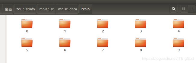
10000张图片, 用于测试。
每个图片都有28×28个像素:

实在搞不定的同学去我百度盘下载吧:
链接: https://pan.baidu.com/s/17WCZ1UABVOuHblsimAZFKw 提取码: 4a8m
解压出来就是这样:

记得刷666。
2.生成了txt列表清单(train.txt和test.txt):
-
为什么要做图片清单?
因为要在训练模型的时候,它们需要学习,就需要根据这个清单,去把图片归类,归到属于它的标识符,然后就记住了这个标识符,最后识别的时候就根据这个去匹配,最后告诉人们这是什么东西?
针对于数据集少的时候,我们可以手动制作图片清单,但是如果数据集很大,比如现在,6w多张图片,这就需要写一个python或者sh脚本(windows下bat文件)来完成了。
新建一个python脚本:
源码:
#-*- coding:utf-8 -*-
# author zoutao
# 2017/11/2
import os
def caffe_input_txt_maker(data_folder,outfile_name, phase = 'train'):
    # 计数文件个数
    file_cnt = 0
    class_cnt = 0
    with open(outfile_name,'w') as fobj:
        for folder_name in os.listdir(data_folder):
            label = folder_name.split('__')[0]
            folder_path = os.path.join(data_folder, folder_name)
            class_cnt += 1
            for file_name in os.listdir(folder_path):
                file_cnt +=1
                # 将文件夹名称也添加入内
                if phase == 'train' :
                    file_path = 'mnist_zt/mnist_data/train/' + folder_name + '/' + file_name
                if phase == 'test' :
                    file_path = 'mnist_zt/mnist_data/test/' + folder_name + '/' + file_name
		#空格一定只要一个就行
                fobj.writelines( file_path +" "+str(label)+'\n')
    file_dir, base_name = os.path.split(outfile_name)
    file_name, ext = os.path.splitext(base_name)
    new_outfile_name = file_dir + '/' + file_name + '_%d_%d' % (class_cnt, file_cnt) + ext
    if os.path.exists(new_outfile_name):
        os.remove(new_outfile_name)
    os.rename(outfile_name, new_outfile_name)
    print ('Done')

if __name__ == "__main__":
    caffe_input_txt_maker(data_folder = 'mnist_data/train',
                         outfile_name = "./train.txt", phase = 'train')

    caffe_input_txt_maker(data_folder = 'mnist_data/test',
                         outfile_name = "./test.txt", phase = 'test')
在caffe/mnis下运行该脚本文件,
python mnist_list.py
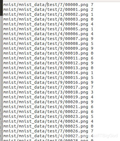
即可得到list;
如图:
训练集:train.txt

测试集:test.txt
此处注意:一般caffe程序都是先将图片转换成lmdb文件,但这样做有点麻烦。因此我就不转换了,我直接用原始图片进行操作,所不同的就是直接用图片操作,均值很难计算,因此可以不减均值,最多就是精度下降一些,训练慢一下;(本例中没有减去均值)。
3.生成参数文件solver
目前已经有了train.txt 和test.txt文件,其他还需要自己编写的有三个文件:train.prototxt,test.prototxt,solver.prototxt
模型就用程序自带的LeNet模型,位置在 ./caffe/models/bvlc_googlenet/文件夹下, 将需要的两个配置文件solver.prototxt和train_val.prototxt,复制到mnist文件夹内:
首先我们修改的是solver.prototxt文件:
sudo vi examples/mnist/solver.prototxt
修改成为如下:
train_net: "/home/zoutao/mnist/train.prototxt"
test_net: "/home/zoutao/mnist/test.prototxt"
test_iter: 100
test_interval: 938
base_lr: 0.01
display: 20
max_iter: 9380
lr_policy: "step"
gamma: 0.1
momentum: 0.9
weight_decay: 0.0005
stepsize: 3000
snapshot: 938
snapshot_prefix: "/home/zoutao/mnist/lenet"
solver_mode: GPU
type: "SGD"
60000条数据,batch_size为64,因此test_iter设置为938,就能全cover了。在训练过程中,调整学习率base_lr,逐步变小。
上面这个文件,你可以在编辑器里面直接书写,也可以用python来生成。
生成参数文件solver代码:
#编写一个函数,生成参数文件
def gen_solver(solver_file,train_net,test_net):
    s=proto.caffe_pb2.SolverParameter()
    s.train_net =train_net
    s.test_net.append(test_net)
    s.test_interval = 938    #60000/64,测试间隔参数:训练完一次所有的图片,进行一次测试
    s.test_iter.append(100)  #10000/100 测试迭代次数,需要迭代100次,才完成一次所有数据的测试
    s.max_iter = 9380       #10 epochs , 938*10,最大训练次数
    s.base_lr = 0.01    #基础学习率
    s.momentum = 0.9    #动量
    s.weight_decay = 5e-4  #权值衰减项
    s.lr_policy = 'step'   #学习率变化规则
    s.stepsize=3000         #学习率变化频率
    s.gamma = 0.1          #学习率变化指数
    s.display = 20         #屏幕显示间隔
    s.snapshot = 938       #保存caffemodel的间隔
    s.snapshot_prefix =root+'mnist/lenet'   #caffemodel前缀
    s.type ='SGD'         #优化算法
    s.solver_mode = proto.caffe_pb2.SolverParameter.GPU    #加速
    #写入solver.prototxt
    with open(solver_file, 'w') as f:
        f.write(str(s))
这样也会产生我们需要的solver.prototxt文件。上面方法二选一。
4.生成配置文件train.prototxt
接下里是train_val.prototxt的改写,因为我们把训练集和测试集分开了,而且做的是两个不同的清单,所以我们将train_val.prototxt拆分为
train.prototxt和test.prototxt两个文件。
首先是 train.prototxt,因我们的数据集是图片,而不是lmdb数据集。所以需要修改两个阶段的data层,实际上修改两个data layer的mean_file和source这两个地方,其它结构可以不用管。
修改后源码:
layer {
  name: "ImageData1"
  type: "ImageData"
  top: "ImageData1"
  top: "ImageData2"
  transform_param {
    scale: 0.00390625
  }
  image_data_param {
    source: "/home/zoutao/mnist/mnist_data/train/train.txt"
    batch_size: 64
    root_folder: "/home/zoutao/"
  }
}
layer {
  name: "Convolution1"
  type: "Convolution"
  bottom: "ImageData1"
  top: "Convolution1"
  convolution_param {
    num_output: 20
    pad: 0
    kernel_size: 5
    stride: 1
    weight_filler {
      type: "xavier"
    }
  }
}
layer {
  name: "Pooling1"
  type: "Pooling"
  bottom: "Convolution1"
  top: "Pooling1"
  pooling_param {
    pool: MAX
    kernel_size: 2
    stride: 2
  }
}
layer {
  name: "Convolution2"
  type: "Convolution"
  bottom: "Pooling1"
  top: "Convolution2"
  convolution_param {
    num_output: 50
    pad: 0
    kernel_size: 5
    stride: 1
    weight_filler {
      type: "xavier"
    }
  }
}
layer {
  name: "Pooling2"
  type: "Pooling"
  bottom: "Convolution2"
  top: "Pooling2"
  pooling_param {
    pool: MAX
    kernel_size: 2
    stride: 2
  }
}
layer {
  name: "InnerProduct1"
  type: "InnerProduct"
  bottom: "Pooling2"
  top: "InnerProduct1"
  inner_product_param {
    num_output: 500
    weight_filler {
      type: "xavier"
    }
  }
}
layer {
  name: "ReLU1"
  type: "ReLU"
  bottom: "InnerProduct1"
  top: "InnerProduct1"
}
layer {
  name: "InnerProduct2"
  type: "InnerProduct"
  bottom: "InnerProduct1"
  top: "InnerProduct2"
  inner_product_param {
    num_output: 10
    weight_filler {
      type: "xavier"
    }
  }
}
layer {
  name: "SoftmaxWithLoss1"
  type: "SoftmaxWithLoss"
  bottom: "InnerProduct2"
  bottom: "ImageData2"
  top: "SoftmaxWithLoss1"
}
图:

后面是test.prototxt:
也是需要修改date层:
源码:
layer {
  name: "ImageData1"
  type: "ImageData"
  top: "ImageData1"
  top: "ImageData2"
  transform_param {
    scale: 0.00390625
  }
  image_data_param {
    source: "/home/zoutao/mnist/mnist_data/test/test.txt"
    batch_size: 100
    root_folder: "/home/zoutao/"
  }
}
layer {
  name: "Convolution1"
  type: "Convolution"
  bottom: "ImageData1"
  top: "Convolution1"
  convolution_param {
    num_output: 20
    pad: 0
    kernel_size: 5
    stride: 1
    weight_filler {
      type: "xavier"
    }
  }
}
layer {
  name: "Pooling1"
  type: "Pooling"
  bottom: "Convolution1"
  top: "Pooling1"
  pooling_param {
    pool: MAX
    kernel_size: 2
    stride: 2
  }
}
layer {
  name: "Convolution2"
  type: "Convolution"
  bottom: "Pooling1"
  top: "Convolution2"
  convolution_param {
    num_output: 50
    pad: 0
    kernel_size: 5
    stride: 1
    weight_filler {
      type: "xavier"
    }
  }
}
layer {
  name: "Pooling2"
  type: "Pooling"
  bottom: "Convolution2"
  top: "Pooling2"
  pooling_param {
    pool: MAX
    kernel_size: 2
    stride: 2
  }
}
layer {
  name: "InnerProduct1"
  type: "InnerProduct"
  bottom: "Pooling2"
  top: "InnerProduct1"
  inner_product_param {
    num_output: 500
    weight_filler {
      type: "xavier"
    }
  }
}
layer {
  name: "ReLU1"
  type: "ReLU"
  bottom: "InnerProduct1"
  top: "InnerProduct1"
}
layer {
  name: "InnerProduct2"
  type: "InnerProduct"
  bottom: "InnerProduct1"
  top: "InnerProduct2"
  inner_product_param {
    num_output: 10
    weight_filler {
      type: "xavier"
    }
  }
}
layer {
  name: "SoftmaxWithLoss1"
  type: "SoftmaxWithLoss"
  bottom: "InnerProduct2"
  bottom: "ImageData2"
  top: "SoftmaxWithLoss1"
}
layer {
  name: "Accuracy1"
  type: "Accuracy"
  bottom: "InnerProduct2"
  bottom: "ImageData2"
  top: "Accuracy1"
}
图:

如果有人想知道为什么这么修改或者是每层都什么意思?
后面的文章会进行讲解。
上面是手动写的方式,可以直接到编辑器里编写,当然也可以用代码生成。
用python来生成源码:
#编写一个函数,生成配置文件prototxt
def Lenet(img_list,batch_size,include_acc=False):
    #第一层,数据输入层,以ImageData格式输入
    data, label = L.ImageData(source=img_list, batch_size=batch_size, ntop=2,root_folder=root,
        transform_param=dict(scale= 0.00390625))
    #第二层:卷积层
    conv1=L.Convolution(data, kernel_size=5, stride=1,num_output=20, pad=0,weight_filler=dict(type='xavier'))
    #池化层
    pool1=L.Pooling(conv1, pool=P.Pooling.MAX, kernel_size=2, stride=2)
    #卷积层
    conv2=L.Convolution(pool1, kernel_size=5, stride=1,num_output=50, pad=0,weight_filler=dict(type='xavier'))
    #池化层
    pool2=L.Pooling(conv2, pool=P.Pooling.MAX, kernel_size=2, stride=2)
    #全连接层
    fc3=L.InnerProduct(pool2, num_output=500,weight_filler=dict(type='xavier'))
    #激活函数层
    relu3=L.ReLU(fc3, in_place=True)
    #全连接层
    fc4 = L.InnerProduct(relu3, num_output=10,weight_filler=dict(type='xavier'))
    #softmax层
    loss = L.SoftmaxWithLoss(fc4, label)

    if include_acc:             # test阶段需要有accuracy层
        acc = L.Accuracy(fc4, label)
        return to_proto(loss, acc)
    else:
        return to_proto(loss)

def write_net():
    #写入train.prototxt
    with open(train_proto, 'w') as f:
        f.write(str(Lenet(train_list,batch_size=64)))

    #写入test.prototxt
    with open(test_proto, 'w') as f:
        f.write(str(Lenet(test_list,batch_size=100, include_acc=True)))
但是要注意我们这里生成的network,可能和原始的Lenet不太一样,不过影响不大。
4.训练mnist的模型
我们需要采用caffe自带的工具来进行训练。
可以采用命令行的形式执行:
sudo build/tools/caffe train -solver examples/mnist/solver.prototxt
也可以采用python脚本来执行训练操作:
源码:
#开始训练
def training(solver_proto):
    caffe.set_device(0)
    caffe.set_mode_gpu()
    solver = caffe.SGDSolver(solver_proto)
    solver.solve()
训练过程中,也会不停的测试哟。
注意:(鉴于很多人不会sh脚本和caffe不熟悉)
上面给的python脚本都是分散的函数。
最终整合在一起才是完整的从生成配置文件+网络参数+模型训练的脚本:
mnist_model_train.py源码:
# -*- coding: utf-8 -*-

# zoutao
# 2017/11/2

import caffe
from caffe import layers as L,params as P,proto,to_proto
#设定文件的保存路径
root='/home/zoutao/'                           #根目录
train_list=root+'mnist/mnist_data/train/train.txt'     #训练图片列表
test_list=root+'mnist/mnist_data/test/test.txt'        #测试图片列表
train_proto=root+'mnist/train.prototxt'     #训练配置文件
test_proto=root+'mnist/test.prototxt'       #测试配置文件
solver_proto=root+'mnist/solver.prototxt'   #参数文件

#编写一个函数,生成配置文件prototxt
def Lenet(img_list,batch_size,include_acc=False):
    #第一层,数据输入层,以ImageData格式输入
    data, label = L.ImageData(source=img_list, batch_size=batch_size, ntop=2,root_folder=root,
        transform_param=dict(scale= 0.00390625))
    #第二层:卷积层
    conv1=L.Convolution(data, kernel_size=5, stride=1,num_output=20, pad=0,weight_filler=dict(type='xavier'))
    #池化层
    pool1=L.Pooling(conv1, pool=P.Pooling.MAX, kernel_size=2, stride=2)
    #卷积层
    conv2=L.Convolution(pool1, kernel_size=5, stride=1,num_output=50, pad=0,weight_filler=dict(type='xavier'))
    #池化层
    pool2=L.Pooling(conv2, pool=P.Pooling.MAX, kernel_size=2, stride=2)
    #全连接层
    fc3=L.InnerProduct(pool2, num_output=500,weight_filler=dict(type='xavier'))
    #激活函数层
    relu3=L.ReLU(fc3, in_place=True)
    #全连接层
    fc4 = L.InnerProduct(relu3, num_output=10,weight_filler=dict(type='xavier'))
    #softmax层
    loss = L.SoftmaxWithLoss(fc4, label)

    if include_acc:             # test阶段需要有accuracy层
        acc = L.Accuracy(fc4, label)
        return to_proto(loss, acc)
    else:
        return to_proto(loss)

def write_net():
    #写入train.prototxt
    with open(train_proto, 'w') as f:
        f.write(str(Lenet(train_list,batch_size=64)))

    #写入test.prototxt
    with open(test_proto, 'w') as f:
        f.write(str(Lenet(test_list,batch_size=100, include_acc=True)))

#编写一个函数,生成参数文件
def gen_solver(solver_file,train_net,test_net):
    s=proto.caffe_pb2.SolverParameter()
    s.train_net =train_net
    s.test_net.append(test_net)
    s.test_interval = 938    #60000/64,测试间隔参数:训练完一次所有的图片,进行一次测试
    s.test_iter.append(100)  #10000/100 测试迭代次数,需要迭代100次,才完成一次所有数据的测试
    s.max_iter = 9380       #10 epochs , 938*10,最大训练次数
    s.base_lr = 0.01    #基础学习率
    s.momentum = 0.9    #动量
    s.weight_decay = 5e-4  #权值衰减项
    s.lr_policy = 'step'   #学习率变化规则
    s.stepsize=3000         #学习率变化频率
    s.gamma = 0.1          #学习率变化指数
    s.display = 20         #屏幕显示间隔
    s.snapshot = 938       #保存caffemodel的间隔
    s.snapshot_prefix = root+'mnist/lenet'   #caffemodel前缀
    s.type ='SGD'         #优化算法
    s.solver_mode = proto.caffe_pb2.SolverParameter.GPU    #加速
    #写入solver.prototxt
    with open(solver_file, 'w') as f:
        f.write(str(s))

#开始训练
def training(solver_proto):
    caffe.set_device(0)
    caffe.set_mode_gpu()
    solver = caffe.SGDSolver(solver_proto)
    solver.solve()
#
if __name__ == '__main__':
    write_net()
    gen_solver(solver_proto,train_proto,test_proto)
    training(solver_proto)
终端运行该py文件:
python mnist_model_train.py
就会开始生成文件train.prototxt,test.prototxt,solver.prototxt和执行模型训练。
采用命令行执行和采用py脚本执行效果是一样的。
模型训练结果:
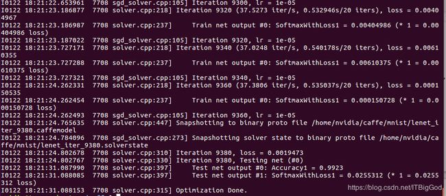
运行时间和最后的精确度,会根据机器配置,参数设置的不同而不同。我的是gpu+cudnn运行我设置训练10 epoch,9000多次,测试精度可以达到99.23%;
而且,在mnist文件夹下,生成了lenet_iter_9380.caffemodel,这个就是我们训练好的模型文件。

5.用训练好的模型来分类识别新的图片:
如果要把训练好的模型拿来测试新的图片,那必须得要一个deploy.prototxt文件,这个文件实际上和test.prototxt文件差不多,只是头尾不相同而也。
deploy文件没有第一层数据输入层,也没有最后的Accuracy层,但最后多了一个Softmax概率层。
在这里我用了python来生成:
1.新建 deploy.py生成deploy.prototxt:
# -*- coding: utf-8 -*-

# zoutao
# 2017/11/2

import caffe
from caffe import layers as L,params as P,to_proto
root='/home/zoutao/'
deploy=root+'mnist/deploy.prototxt'    #文件保存路径

def create_deploy():
    #少了第一层,data层
    conv1=L.Convolution(bottom='data', kernel_size=5, stride=1,num_output=20, pad=0,weight_filler=dict(type='xavier'))
    pool1=L.Pooling(conv1, pool=P.Pooling.MAX, kernel_size=2, stride=2)
    conv2=L.Convolution(pool1, kernel_size=5, stride=1,num_output=50, pad=0,weight_filler=dict(type='xavier'))
    pool2=L.Pooling(conv2, pool=P.Pooling.MAX, kernel_size=2, stride=2)
    fc3=L.InnerProduct(pool2, num_output=500,weight_filler=dict(type='xavier'))
    relu3=L.ReLU(fc3, in_place=True)
    fc4 = L.InnerProduct(relu3, num_output=10,weight_filler=dict(type='xavier'))
    #最后没有accuracy层,但有一个Softmax层
    prob=L.Softmax(fc4)
    return to_proto(prob)
def write_deploy():
    with open(deploy, 'w') as f:
        f.write('name:"Lenet"\n')
        f.write('input:"data"\n')
        f.write('input_dim:1\n')
        f.write('input_dim:3\n')
        f.write('input_dim:28\n')
        f.write('input_dim:28\n')
        f.write(str(create_deploy()))
if __name__ == '__main__':
    write_deploy()
这样就生成了一个deploy.prototxt文件。
生成不了的,给出源码,复制即可。
deploy.prototxt源码:
name:"Lenet"
input:"data"
input_dim:1
input_dim:3
input_dim:28
input_dim:28
layer {
  name: "Convolution1"
  type: "Convolution"
  bottom: "data"
  top: "Convolution1"
  convolution_param {
    num_output: 20
    pad: 0
    kernel_size: 5
    stride: 1
    weight_filler {
      type: "xavier"
    }
  }
}
layer {
  name: "Pooling1"
  type: "Pooling"
  bottom: "Convolution1"
  top: "Pooling1"
  pooling_param {
    pool: MAX
    kernel_size: 2
    stride: 2
  }
}
layer {
  name: "Convolution2"
  type: "Convolution"
  bottom: "Pooling1"
  top: "Convolution2"
  convolution_param {
    num_output: 50
    pad: 0
    kernel_size: 5
    stride: 1
    weight_filler {
      type: "xavier"
    }
  }
}
layer {
  name: "Pooling2"
  type: "Pooling"
  bottom: "Convolution2"
  top: "Pooling2"
  pooling_param {
    pool: MAX
    kernel_size: 2
    stride: 2
  }
}
layer {
  name: "InnerProduct1"
  type: "InnerProduct"
  bottom: "Pooling2"
  top: "InnerProduct1"
  inner_product_param {
    num_output: 500
    weight_filler {
      type: "xavier"
    }
  }
}
layer {
  name: "ReLU1"
  type: "ReLU"
  bottom: "InnerProduct1"
  top: "InnerProduct1"
}
layer {
  name: "InnerProduct2"
  type: "InnerProduct"
  bottom: "InnerProduct1"
  top: "InnerProduct2"
  inner_product_param {
    num_output: 10
    weight_filler {
      type: "xavier"
    }
  }
}
layer {
  name: "Softmax1"
  type: "Softmax"
  bottom: "InnerProduct2"
  top: "Softmax1"
}
2.分类标签lables.txt文件:
还需要写一个分类标签lables.txt文件,这个文件不推荐用代码来生成,反而麻烦。
在图片清单的地方,加上一个标签类:labels.txt,让模型知道分为几类,从而去根据图片匹配属于的类型,我们有一个train.txt和test.txt而且放在不同的地方,
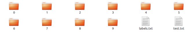
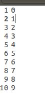
在test跟train下,分别新建一个label.txt标签,写好分类情况:
图:

注意:是test跟train都分别写一个lable.txt文件;
标签文件内容为:0-9 ,
3.挑选图片准备测试:
我们从mnist数据集的test集中随便找一张图片,用来进行分类识别的实验。
比如:

当然,如果你想自己搞一个图片也可以,
打开Windows自带的画图工具,新建三张图片,调整像素大小均为28*28;分别用画笔写上数字0、4、8,分别保存为png、jpg、bmp格式,即得到三个手写数字:
图示:

4.测试图片识别
实现模型测试样本识别有两种常用方式:
- 第一种采用命令行的形式。
- 第二种使用python接口。
使用命令行的方式运行图片识别测试:
./build/examples/cpp_classification/classification.bin mnist/deploy.prototxt mnist_zt/caffenet_iter_9380.caffemodel mnist/mnist_data/test/labels.txt mnist_zt/mnist_data/test/6/00011.png
本例子会提示:

这是却少参数了。
命令行调用caffe工具预测是需要有6个参数:
-
1.classification.bin caffe自带的bin工具
-
2.deploy.prototxt 网络配置文件
-
3.network.caffemodel 训练好的模型文件
-
4.mean.binaryproto 均值文件
-
5.labels.txt 标签文本
-
6.img.jpg 测试的图片
由于本项目中我们没有写均值文件,所以这里直接这么写是没法使用的。
第二种方式:
编写一个test_one.py文件:
#coding=utf-8
# zoutao
# 2017/11/2

import caffe
import numpy as np
root='/home/zoutao/caffe/examples/'   #根目录
deploy=root + 'mnist/deploy.prototxt'    #deploy文件
caffe_model=root + 'mnist/lenet_iter_9380.caffemodel'   #训练好的 caffemodel
img=root+'mnist/mnist_data/test/6/00006.png'    #随机找的一张待测图片
labels_filename = root + 'mnist/mnist_data/test/labels.txt'  #类别名称文件,将数字标签转换回类别名称

net = caffe.Net(deploy,caffe_model,caffe.TEST)   #加载model和network

#图片预处理设置
transformer = caffe.io.Transformer({'data': net.blobs['data'].data.shape})  #设定图片的shape格式(1,3,28,28)
transformer.set_transpose('data', (2,0,1))    #改变维度的顺序,由原始图片(28,28,3)变为(3,28,28)
#transformer.set_mean('data', np.load(mean_file).mean(1).mean(1))    #减去均值,前面训练模型时没有减均值,这儿就不用
#im -= np.array((104.00698793,116.66876762,122.67891434)) #可以手动计算均值,并减去
transformer.set_raw_scale('data', 255)    # 缩放到【0,255】之间
transformer.set_channel_swap('data', (2,1,0))   #交换通道,将图片由RGB变为BGR

im=caffe.io.load_image(img)                   #加载图片
net.blobs['data'].data[...] = transformer.preprocess('data',im)      #执行上面设置的图片预处理操作,并将图片载入到blob中

#执行测试
out = net.forward()

labels = np.loadtxt(labels_filename, str, delimiter='\t')   #读取类别名称文件
prob= net.blobs['Softmax1'].data[0].flatten() #取出最后一层(Softmax)属于某个类别的概率值,并打印
print prob
order=prob.argsort()[-1]  #将概率值排序,取出最大值所在的序号
print 'the class is:',labels[order]   #将该序号转换成对应的类别名称,并打印
然后运行该py文件,最后结果:
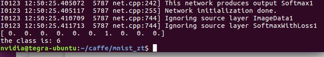
最后输出 the class is : 6 ,分类正确。
如果是预测多张图片,可把上面这个文件写成一个函数,然后进行循环预测就可以了。
好啦以上就是整个开发mnist手写体识别项目的过程,虽然比较简单,但是深度学习入门基本上都是以mnist为例子,举一反三的做法。
常见报错总结:
问题一:分类识别的时候出现这个:nan值
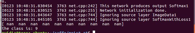
loss随着每轮迭代越来越大,最终超过了浮点型表示的范围,就变成了NaN。
措施:
- 减小solver.prototxt中的base_lr,至少减小一个数量级。如果解决不了,
则再如果有多个loss layer,需要找出哪个损失层导致了梯度爆炸,并在train_val.prototxt中减小该层的loss_weight,而非是减小通用的base_lr。 - 设置clip gradient,用于限制过大的diff
- 其次就是你要去看是不是你的txt文本不是int类型或者是list清单中没有乱序,这样也会导致你训练时候精度一直是等于1;
问题二:在使用自己的参数进行训练的过程中发现,loss的值或者输出值非常大或者显示成NaN或inf的时候。
这说明你的学习过程发散了,这是应该降低base_lr(修改学习率)重新训练,知道你找到了一个合适的base_lr为止。
问题三:如果你训练的结果中:出现了loss=87.3365,或者 是SoftmaxWithLoss = 87.3362,
前面几十次迭代loss是很小的数值,迭代一百多次就变成固定值87.3365。
解决:
调整学习率,一般是先从0.1开始,每一次由0.05,0.01,0.005,0.001……调小,如果一直都是这个数,就要考虑一下数据集和去检查你的图片清单有没有做成乱序的,或者是清单中名称跟数字之间是不是只有一个空格隔开;
问题四:如果你是拿别人的modles来做微调finetune时候也会出现这样的问题–是因为分类层的 num_output 和 标签的值域不符合:
a. 要知道imagenet是进行1000类的分类任务,我自己的数据是一个二分类,就一定要把最后‘fc8’InnerProduct的分类层的num_output: 2 原来是1000,这个设成自己label的类别总数就可以。
b. 但是注意同时要修改train.prototxt和deploy.prototxt两个网络配置文件中的num_output。
参考网站:
图层解释:https://blog.csdn.net/real_myth/article/details/51180569
windwos下版本:https://blog.csdn.net/u012958854/article/details/78193551