Coursera吴恩达Deep Learning.ai第一课第四周Building your Deep Neural Network: Step by Step

 

Building your Deep Neural Network: Step by Step

您将构建一个深层神经网络，拥有您想要的多个层！
完成此任务后，您将能够：

• 使用ReLU等非线性单位来改善您的模型。
• 构建更深层的神经网络（具有多于1个隐藏层）。
• 实现易于使用的神经网络类。

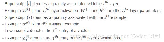
符号：

1 - 包

• numpy是使用Python进行科学计算的主要软件包。
• matplotlib是一个用Python绘制图形的库。
• dnn_utils为这款笔记本提供了一些必要的功能。
• testCases提供了一些测试用例来评估函数的正确性
• np.random.seed（1）用于保持所有随机函数调用一致。 它将帮助我们评估您的工作。 请不要改变种子。

import numpy as np
import h5py
import matplotlib.pyplot as plt
from testCases import *
from dnn_utils import sigmoid, sigmoid_backward, relu, relu_backward

%matplotlib inline
plt.rcParams['figure.figsize'] = (5.0, 4.0) # set default size of plots
plt.rcParams['image.interpolation'] = 'nearest'
plt.rcParams['image.cmap'] = 'gray'

%load_ext autoreload
%autoreload 2

np.random.seed(1)

 

2 - 作业概要

要构建您的神经网络，您将实现几个“辅助函数”。这些辅助函数将用于下一个任务，以构建一个双层神经网络和一个L层神经网络。以下是此作业的概要，您将：

• 初始化双层网络和L层神经网络的参数。
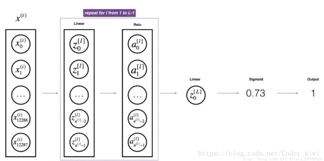
• 实现前向传播模块（如下图中的紫色所示）。

• 完成图层前向传播步骤的LINEAR部分（得到Z [1]）。

• 我们为您提供ACTIVATION功能（relu / sigmoid）。

• 将前两个步骤组合成一个新的[LINEAR-> ACTIVATION]前向功能。

• 堆叠[LINEAR-> RELU]前向功能L-1时间（对于第1层到第L-1层）并在末尾添加[LINEAR-> SIGMOID]（对于最后一层L）。这为您提供了一个新的L_model_forward函数。

• 计算损失。
• 实现后向传播模块（下图中以红色表示）。
• 完成图层向后传播步骤的LINEAR部分。

• 我们给你ACTIVATE函数的渐变（relu_backward / sigmoid_backward）

• 将前两个步骤组合成一个新的[LINEAR-> ACTIVATION]向后功能。

• 向后堆叠[LINEAR-> RELU] L-1次并在新的L_model_backward函数中向后添加[LINEAR-> SIGMOID]

• 最后更新参数。

 

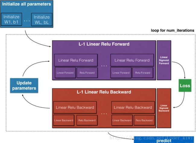
注意：对于每个前向功能，都有相应的后向功能。在转发模块的每一步中，您都会将一些值存储在缓存中。缓存的值对计算渐变很有用。在反向传播模块中，您将使用缓存来计算渐变。此作业将向您显示如何执行这些步骤。

3 - 初始化

您将编写两个辅助函数来初始化模型的参数。第一个函数将用于初始化双层模型的参数。第二个将把这个初始化过程推广到L层。

3.1 - 2层神经网络

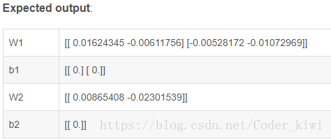
练习：创建并初始化2层神经网络的参数。

说明：

• 模型的结构是：LINEAR - > RELU - > LINEAR - > SIGMOID。
• 对权重矩阵使用随机初始化。使用正确形状的np.random.randn（shape）* 0.01。
• 对偏差使用零初始化。使用np.zeros（shape）。

# GRADED FUNCTION: initialize_parameters

def initialize_parameters(n_x, n_h, n_y):
    """
    Argument:
    n_x -- size of the input layer
    n_h -- size of the hidden layer
    n_y -- size of the output layer

    Returns:
    parameters -- python dictionary containing your parameters:
                    W1 -- weight matrix of shape (n_h, n_x)
                    b1 -- bias vector of shape (n_h, 1)
                    W2 -- weight matrix of shape (n_y, n_h)
                    b2 -- bias vector of shape (n_y, 1)
    """

    np.random.seed(1)

    ### START CODE HERE ### (≈ 4 lines of code)
    W1 = np.random.randn(n_h, n_x) * 0.01
    b1 = np.zeros((n_h, 1))
    W2 = np.random.randn(n_y, n_h) * 0.01
    b2 = np.zeros((n_y, 1))
    ### END CODE HERE ###

    assert(W1.shape == (n_h, n_x))
    assert(b1.shape == (n_h, 1))
    assert(W2.shape == (n_y, n_h))
    assert(b2.shape == (n_y, 1))

    parameters = {"W1": W1,
                  "b1": b1,
                  "W2": W2,
                  "b2": b2}

    return parameters   

parameters = initialize_parameters(2,2,1)
print("W1 = " + str(parameters["W1"]))
print("b1 = " + str(parameters["b1"]))
print("W2 = " + str(parameters["W2"]))
print("b2 = " + str(parameters["b2"]))

 

3.2 - L层神经网络

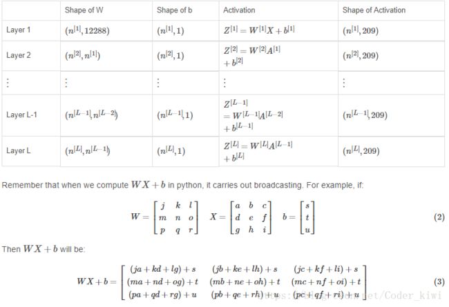
更深层的L层神经网络的初始化更复杂，因为有更多的权重矩阵和偏置向量。 完成initialize_parameters_deep后，您应确保每个图层之间的尺寸匹配。 回想一下，n [l]是层l中的单元数。 因此，例如，如果我们的输入X的大小是（12288,209）（m = 209个例子）那么：

练习：实现L层神经网络的初始化。

说明：

• 模型的结构是[LINEAR - > RELU]×（L-1） - > LINEAR - > SIGMOID。即，它具有L-1层，使用ReLU激活函数，接着是具有S形激活函数的输出层。
• 对权重矩阵使用随机初始化。使用np.random.rand（shape）* 0.01。
• 对偏差使用零初始化。使用np.zeros（shape）。
• 我们将在变量layer_dims中存储n [l]，即不同层中的单元数。例如，上周的“平面数据分类模型”的layer_dims将是[2,4,1]：有两个输入，一个隐藏层有4个隐藏单元，一个输出层有一个输出单元。因此，W1的形状为（4,2），b1为（4,1），W2为（1,4），b2为（1,1）。现在你将它推广到L层！
• 这是L = 1（单层神经网络）的实现。它应该激励你实现一般情况（L层神经网络）。

if L == 1:
        parameters["W" + str(L)] = np.random.randn(layer_dims[1], layer_dims[0]) * 0.01
        parameters["b" + str(L)] = np.zeros((layer_dims[1], 1))

# GRADED FUNCTION: initialize_parameters_deep

def initialize_parameters_deep(layer_dims):
    """
    Arguments:
    layer_dims -- python array (list) containing the dimensions of each layer in our network

    Returns:
    parameters -- python dictionary containing your parameters "W1", "b1", ..., "WL", "bL":
                    Wl -- weight matrix of shape (layer_dims[l], layer_dims[l-1])
                    bl -- bias vector of shape (layer_dims[l], 1)
    """

    np.random.seed(3)
    parameters = {}
    L = len(layer_dims)            # number of layers in the network

    for l in range(1, L):
        ### START CODE HERE ### (≈ 2 lines of code)
        parameters['W' + str(l)] = np.random.randn(layer_dims[l], layer_dims[l - 1]) * 0.01
        parameters['b' + str(l)] = np.zeros((layer_dims[l], 1))
        ### END CODE HERE ###

        assert(parameters['W' + str(l)].shape == (layer_dims[l], layer_dims[l-1]))
        assert(parameters['b' + str(l)].shape == (layer_dims[l], 1))


    return parameters

parameters = initialize_parameters_deep([5,4,3])
print("W1 = " + str(parameters["W1"]))
print("b1 = " + str(parameters["b1"]))
print("W2 = " + str(parameters["W2"]))
print("b2 = " + str(parameters["b2"]))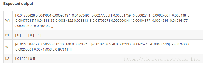

4 - 前向传播模块

4.1 - 线性前向

现在您已经初始化了参数，您将进行前向传播模块。 您将首先实现一些基本功能，稍后您将在实现模型时使用这些功能。 您将按此顺序完成三个功能：

• LINEAR
• LINEAR - > ACTIVATION，其中ACTIVATION将是ReLU或Sigmoid。
• [LINEAR - > RELU]×（L-1） - > LINEAR - > SIGMOID（整个模型）

线性前向模块（在所有示例中矢量化）计算以下等式：

其中

练习：构建前向传播的线性部分。

提醒：该单位的数学表示为。 您可能还会发现np.dot（）很有用。 如果您的尺寸不匹配，打印W.shape可能会有所帮助。

# GRADED FUNCTION: linear_forward

def linear_forward(A, W, b):
    """
    Implement the linear part of a layer's forward propagation.

    Arguments:
    A -- activations from previous layer (or input data): (size of previous layer, number of examples)
    W -- weights matrix: numpy array of shape (size of current layer, size of previous layer)
    b -- bias vector, numpy array of shape (size of the current layer, 1)

    Returns:
    Z -- the input of the activation function, also called pre-activation parameter 
    cache -- a python dictionary containing "A", "W" and "b" ; stored for computing the backward pass efficiently
    """

    ### START CODE HERE ### (≈ 1 line of code)
    Z = np.dot(W, A) + b
    ### END CODE HERE ###

    assert(Z.shape == (W.shape[0], A.shape[1]))
    cache = (A, W, b)

    return Z, cache

A, W, b = linear_forward_test_case()

Z, linear_cache = linear_forward(A, W, b)
print("Z = " + str(Z))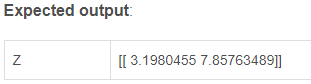

4.2 - 线性激活转发

在此笔记本中，您将使用两个激活功能：

为方便起见，您将把两个函数（线性和激活）分组为一个函数（LINEAR-> ACTIVATION）。 因此，您将实现一个函数，该函数执行LINEAR前进步骤，然后执行ACTIVATION前进步骤。

练习：实现LINEAR-> ACTIVATION图层的前向传播。 数学关系是：其中激活“g”可以是sigmoid（）或relu（）。 使用linear_forward（）和正确的激活函数。

# GRADED FUNCTION: linear_activation_forward

def linear_activation_forward(A_prev, W, b, activation):
    """
    Implement the forward propagation for the LINEAR->ACTIVATION layer

    Arguments:
    A_prev -- activations from previous layer (or input data): (size of previous layer, number of examples)
    W -- weights matrix: numpy array of shape (size of current layer, size of previous layer)
    b -- bias vector, numpy array of shape (size of the current layer, 1)
    activation -- the activation to be used in this layer, stored as a text string: "sigmoid" or "relu"

    Returns:
    A -- the output of the activation function, also called the post-activation value 
    cache -- a python dictionary containing "linear_cache" and "activation_cache";
             stored for computing the backward pass efficiently
    """

    if activation == "sigmoid":
        # Inputs: "A_prev, W, b". Outputs: "A, activation_cache".
        ### START CODE HERE ### (≈ 2 lines of code)
        Z, linear_cache = np.dot(W, A_prev) + b, (A_prev, W, b)
        A, activation_cache = sigmoid(Z)
        ### END CODE HERE ###

    elif activation == "relu":
        # Inputs: "A_prev, W, b". Outputs: "A, activation_cache".
        ### START CODE HERE ### (≈ 2 lines of code)
        Z, linear_cache = np.dot(W, A_prev) + b, (A_prev, W, b)
        A, activation_cache = relu(Z)
        ### END CODE HERE ###

    assert (A.shape == (W.shape[0], A_prev.shape[1]))
    cache = (linear_cache, activation_cache)

    return A, cache

A_prev, W, b = linear_activation_forward_test_case()

A, linear_activation_cache = linear_activation_forward(A_prev, W, b, activation = "sigmoid")
print("With sigmoid: A = " + str(A))

A, linear_activation_cache = linear_activation_forward(A_prev, W, b, activation = "relu")
print("With ReLU: A = " + str(A))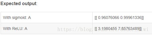

注意：在深度学习中，“[LINEAR-> ACTIVATION]”计算在神经网络中计为单层，而不是两层。

d）L层模型

为了在实现L层神经网络时更加方便，您需要一个能够复制前一个（使用RELU的linear_activation_forward）L-1次的函数，然后使用一个带有SIGMOID的linear_activation_forward。

练习：实现上述模型的前向传播。

指令：在下面的代码中，变量AL将表示。（有时也称为Yhat，即这是。）

提示：

• 使用您之前编写的功能。
• 使用for循环复制[LINEAR-> RELU]（L-1）次。
• 不要忘记跟踪“缓存”列表中的缓存。 要向列表中添加新值c，可以使用list.append（c）。

# GRADED FUNCTION: L_model_forward

def L_model_forward(X, parameters):
    """
    Implement forward propagation for the [LINEAR->RELU]*(L-1)->LINEAR->SIGMOID computation

    Arguments:
    X -- data, numpy array of shape (input size, number of examples)
    parameters -- output of initialize_parameters_deep()

    Returns:
    AL -- last post-activation value
    caches -- list of caches containing:
                every cache of linear_relu_forward() (there are L-1 of them, indexed from 0 to L-2)
                the cache of linear_sigmoid_forward() (there is one, indexed L-1)
    """

    caches = []
    A = X
    L = len(parameters) // 2                  # number of layers in the neural network

    # Implement [LINEAR -> RELU]*(L-1). Add "cache" to the "caches" list.
    for l in range(1, L):
        A_prev = A 
        ### START CODE HERE ### (≈ 2 lines of code)
        A, cache = linear_activation_forward(A_prev, parameters['W' + str(l)], parameters['b' + str(l)], activation = "relu")
        caches.append(cache)
        ### END CODE HERE ###

    # Implement LINEAR -> SIGMOID. Add "cache" to the "caches" list.
    ### START CODE HERE ### (≈ 2 lines of code)
    AL, cache = linear_activation_forward(A, parameters['W' + str(L)], parameters['b' + str(L)], activation = "sigmoid")
    caches.append(cache)

    ### END CODE HERE ###

    assert(AL.shape == (1,X.shape[1]))

    return AL, caches

X, parameters = L_model_forward_test_case()
AL, caches = L_model_forward(X, parameters)
print("AL = " + str(AL))
print("Length of caches list = " + str(len(caches)))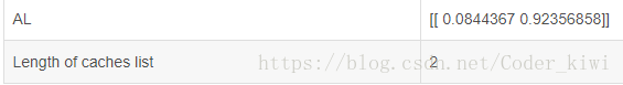

‘

现在，您有一个完整的前向传播，它接受输入X并输出包含您的预测的行向量。 它还记录“caches”中的所有中间值。 使用，您可以计算预测的成本。

5 - 成本函数

现在，您将实现向前和向后传播。 您需要计算成本，因为您要检查您的模型是否实际学习。

练习：使用以下公式计算交叉熵成本J：

# GRADED FUNCTION: compute_cost

def compute_cost(AL, Y):
    """
    Implement the cost function defined by equation (7).

    Arguments:
    AL -- probability vector corresponding to your label predictions, shape (1, number of examples)
    Y -- true "label" vector (for example: containing 0 if non-cat, 1 if cat), shape (1, number of examples)

    Returns:
    cost -- cross-entropy cost
    """

    m = Y.shape[1]

    # Compute loss from aL and y.
    ### START CODE HERE ### (≈ 1 lines of code)
    cost = -1./m * np.sum(Y * np.log(AL) + (1 - Y) * np.log(1 - AL))
    ### END CODE HERE ###

    cost = np.squeeze(cost)      # To make sure your cost's shape is what we expect (e.g. this turns [[17]] into 17).
    assert(cost.shape == ())

    return cost

Y, AL = compute_cost_test_case()

print("cost = " + str(compute_cost(AL, Y)))

6 - 后向传播模块

就像前向传播一样，您将实现反向传播的辅助函数。 请记住，反向传播用于计算损失函数相对于参数的梯度。

提醒:

现在，类似于前向传播，您将分三个步骤构建向后传播：

• 向后LINEAR。
• LINEAR - > ACTIVATION，ACTIVATION计算ReLU或S形激活的导数。
• [LINEAR - > RELU]×（L-1） - > LINEAR - > SIGMOID向后（整个模型）。

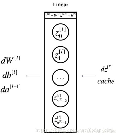
6.1 - 线性向后

对于层l，线性部分是：（随后是激活）。

假设您已经计算了导数。 你想得到。

 

 

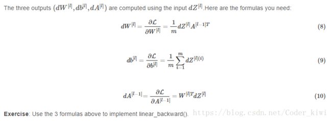
# GRADED FUNCTION: linear_backward

def linear_backward(dZ, cache):
    """
    Implement the linear portion of backward propagation for a single layer (layer l)

    Arguments:
    dZ -- Gradient of the cost with respect to the linear output (of current layer l)
    cache -- tuple of values (A_prev, W, b) coming from the forward propagation in the current layer

    Returns:
    dA_prev -- Gradient of the cost with respect to the activation (of the previous layer l-1), same shape as A_prev
    dW -- Gradient of the cost with respect to W (current layer l), same shape as W
    db -- Gradient of the cost with respect to b (current layer l), same shape as b
    """
    A_prev, W, b = cache
    m = A_prev.shape[1]

    ### START CODE HERE ### (≈ 3 lines of code)
    dW = 1./m * np.dot(dZ, A_prev.T)
    db = 1./m * np.sum(dZ) 
    dA_prev = np.dot(W.T, dZ)
    ### END CODE HERE ###

    assert (dA_prev.shape == A_prev.shape)
    assert (dW.shape == W.shape)
    assert (isinstance(db, float))

    return dA_prev, dW, db

# Set up some test inputs
dZ, linear_cache = linear_backward_test_case()

dA_prev, dW, db = linear_backward(dZ, linear_cache)
print ("dA_prev = "+ str(dA_prev))
print ("dW = " + str(dW))
print ("db = " + str(db))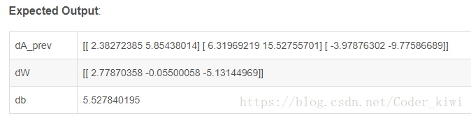

6.2 - 向后线性激活

接下来，您将创建一个合并两个辅助函数的函数：linear_backward和激活linear_activation_backward的后退步骤。

 

# GRADED FUNCTION: linear_activation_backward

def linear_activation_backward(dA, cache, activation):
    """
    Implement the backward propagation for the LINEAR->ACTIVATION layer.

    Arguments:
    dA -- post-activation gradient for current layer l 
    cache -- tuple of values (linear_cache, activation_cache) we store for computing backward propagation efficiently
    activation -- the activation to be used in this layer, stored as a text string: "sigmoid" or "relu"

    Returns:
    dA_prev -- Gradient of the cost with respect to the activation (of the previous layer l-1), same shape as A_prev
    dW -- Gradient of the cost with respect to W (current layer l), same shape as W
    db -- Gradient of the cost with respect to b (current layer l), same shape as b
    """
    linear_cache, activation_cache = cache

    if activation == "relu":
        ### START CODE HERE ### (≈ 2 lines of code)
        dZ = relu_backward(dA, activation_cache)
        dA_prev, dW, db = linear_backward(dZ, linear_cache)
        ### END CODE HERE ###

    elif activation == "sigmoid":
        ### START CODE HERE ### (≈ 2 lines of code)
        dZ = sigmoid_backward(dA, activation_cache)
        dA_prev, dW, db = linear_backward(dZ, linear_cache)
        ### END CODE HERE ###

    return dA_prev, dW, db

AL, linear_activation_cache = linear_activation_backward_test_case()

dA_prev, dW, db = linear_activation_backward(AL, linear_activation_cache, activation = "sigmoid")
print ("sigmoid:")
print ("dA_prev = "+ str(dA_prev))
print ("dW = " + str(dW))
print ("db = " + str(db) + "\n")

dA_prev, dW, db = linear_activation_backward(AL, linear_activation_cache, activation = "relu")
print ("relu:")
print ("dA_prev = "+ str(dA_prev))
print ("dW = " + str(dW))
print ("db = " + str(db))

6.3 - L模型向后

现在，您将为整个网络实现向后功能。回想一下，当您实现L_model_forward函数时，在每次迭代时，您都存储了一个包含（X，W，b和z）的缓存。在反向传播模块中，您将使用这些变量来计算渐变。因此，在L_model_backward函数中，您将从层L开始向后遍历所有隐藏层。在每个步骤中，您将使用层l的缓存值通过层l反向传播。

 

 

# GRADED FUNCTION: L_model_backward

def L_model_backward(AL, Y, caches):
    """
    Implement the backward propagation for the [LINEAR->RELU] * (L-1) -> LINEAR -> SIGMOID group

    Arguments:
    AL -- probability vector, output of the forward propagation (L_model_forward())
    Y -- true "label" vector (containing 0 if non-cat, 1 if cat)
    caches -- list of caches containing:
                every cache of linear_activation_forward() with "relu" (it's caches[l], for l in range(L-1) i.e l = 0...L-2)
                the cache of linear_activation_forward() with "sigmoid" (it's caches[L-1])

    Returns:
    grads -- A dictionary with the gradients
             grads["dA" + str(l)] = ... 
             grads["dW" + str(l)] = ...
             grads["db" + str(l)] = ... 
    """
    grads = {}
    L = len(caches) # the number of layers
    m = AL.shape[1]
    Y = Y.reshape(AL.shape) # after this line, Y is the same shape as AL

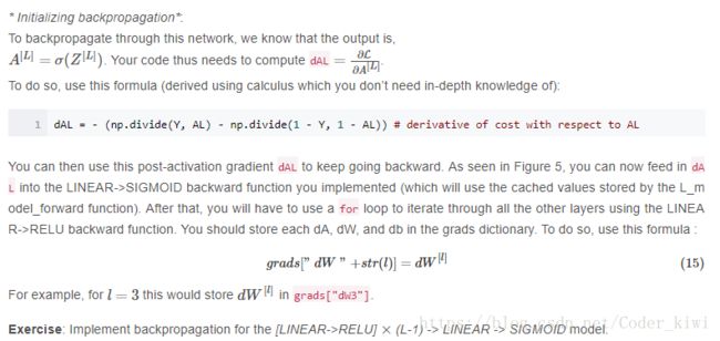
    # Initializing the backpropagation
    ### START CODE HERE ### (1 line of code)
    dAL =  - (np.divide(Y, AL) - np.divide(1 - Y, 1 - AL))
    ### END CODE HERE ###

    # Lth layer (SIGMOID -> LINEAR) gradients. Inputs: "AL, Y, caches". Outputs: "grads["dAL"], grads["dWL"], grads["dbL"]
    ### START CODE HERE ### (approx. 2 lines)
    current_cache = caches[L-1]
    grads["dA" + str(L)], grads["dW" + str(L)], grads["db" + str(L)] = linear_activation_backward(dAL, current_cache, activation = 'sigmoid')
    ### END CODE HERE ###

    for l in reversed(range(L-1)):
        # lth layer: (RELU -> LINEAR) gradients.
        # Inputs: "grads["dA" + str(l + 2)], caches". Outputs: "grads["dA" + str(l + 1)] , grads["dW" + str(l + 1)] , grads["db" + str(l + 1)] 
        ### START CODE HERE ### (approx. 5 lines)
        current_cache = caches[L - 2 - l]
        dA_prev_temp, dW_temp, db_temp = linear_activation_backward(grads["dA" + str(L)], current_cache, activation = 'relu')
        grads["dA" + str(l + 1)] = dA_prev_temp
        grads["dW" + str(l + 1)] = dW_temp
        grads["db" + str(l + 1)] = db_temp
        ### END CODE HERE ###

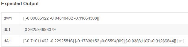
    return grads

X_assess, Y_assess, AL, caches = L_model_backward_test_case()
grads = L_model_backward(AL, Y_assess, caches)
print ("dW1 = "+ str(grads["dW1"]))
print ("db1 = "+ str(grads["db1"]))
print ("dA1 = "+ str(grads["dA1"]))

 

6.4 - 更新参数

在本节中，您将使用渐变下降更新模型的参数：

其中α是学习率。 计算更新的参数后，将它们存储在参数字典中。

练习：使用渐变下降实现update_parameters（）以更新参数。

# GRADED FUNCTION: update_parameters

def update_parameters(parameters, grads, learning_rate):
    """
    Update parameters using gradient descent

    Arguments:
    parameters -- python dictionary containing your parameters 
    grads -- python dictionary containing your gradients, output of L_model_backward

    Returns:
    parameters -- python dictionary containing your updated parameters 
                  parameters["W" + str(l)] = ... 
                  parameters["b" + str(l)] = ...
    """

    L = len(parameters) // 2 # number of layers in the neural network

    # Update rule for each parameter. Use a for loop.
    ### START CODE HERE ### (≈ 3 lines of code)
    for l in range(L):
        parameters["W" + str(l+1)] = parameters["W" + str(l+1)] - learning_rate * grads["dW" + str(l+1)]
        parameters["b" + str(l+1)] = parameters["b" + str(l+1)] - learning_rate * grads["db" + str(l+1)]
    ### END CODE HERE ###

    return parameters

parameters, grads = update_parameters_test_case()
parameters = update_parameters(parameters, grads, 0.1)

print ("W1 = "+ str(parameters["W1"]))
print ("b1 = "+ str(parameters["b1"]))
print ("W2 = "+ str(parameters["W2"]))
print ("b2 = "+ str(parameters["b2"]))
print ("W3 = "+ str(parameters["W3"]))
print ("b3 = "+ str(parameters["b3"]))