基于RNN的时间序列预测
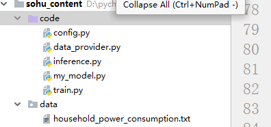
1. 这是整个项目的文件结构
2. 配置文件 config.py
# data_provider: data_power_consumption

path_to_dataset = '../data/household_power_consumption.txt'
sequence_length = 50
ratio= 0.5
epochs = 1

save_path = "../model.h5"
batch_size=512
3. 数据处理文件 data_provider.py
"""
dataset intruduction:
The dataset we'll be using can be downloaded there :
https://archive.ics.uci.edu/ml/datasets/Individual+household+electric+power+consumption#.
It is a 20 Mo zip file containing a text file.

The task here will be to be able to predict values for a timeseries :
the history of 2 million minutes of a household's power consumption.
We are going to use a multi-layered LSTM recurrent neural network
to predict the last value of a sequence of values.
Put another way, given 49 timesteps of consumption, what will be the 50th value?


"""
import matplotlib.pyplot as plt
import numpy as np
import time
import csv
from keras.models import Sequential
from keras.layers.core import Dense, Activation, Dropout
from keras.layers.recurrent import LSTM
np.random.seed(1234)

def data_power_consumption(path_to_dataset, sequence_length, ratio):
    max_values = ratio * 2049280
    with open(path_to_dataset) as f:
        data = csv.reader(f, delimiter = ";")
        power = []
        nb_of_values = 0
        for line in data:
            try:
                power.append(float(line[2]))
                nb_of_values += 1
            except ValueError:
                pass
            # 2049280.0 is the total number of valid values, i.e. ratio = 1.0
            if nb_of_values / 2049280.0 >= ratio:
                break
    """
    The initial file contains lots of different pieces of data.
    We will here focus on a single value : a house's Global_active_power
    history, minute by minute for almost 4 years.
    This means roughly 2 million points.
    Some values are missing, this is why we try to load the values as floats
    into the list and if the value is not a number
    ( missing values are marked with a ?) we simply ignore them.
    Also if we do not want to load the entire dataset,
    there is a condition to stop loading the data
    when a certain ratio is reached.
   """
    result = []
    for index in range(len(power) - sequence_length):
        result.append(power[index: index + sequence_length])
    result = np.array(result) # shape (2049230, 50)

    """
    Once all the datapoints are loaded as one large timeseries,
    we have to split it into examples.
    Again, one example is made of a sequence of 50 values.
    Using the first 49, we are going to try and predict the 50th.
    Moreover, we'll do this for every minute given the 49 previous
    ones so we use a sliding buffer of size 50.
    """
    result_mean = result.mean()
    result -= result_mean
    """
    Neural networks usually learn way better when data is
    pre-processed (cf Y. Lecun's 1995 paper, section 4.3).
    However regarding time-series we do not want the network
    to learn on data too far from the real world.
    So here we'll keep it simple and simply center the data to have a 0 mean.
    """
    row = int(round(0.9 * result.shape[0]))# 行
    train = result[:row, :]
    np.random.shuffle(train)# 按行打乱
    X_train = train[:, :-1]# 49column
    y_train = train[:, -1]# 只有行没有列,就是一列

    X_test = result[row:, :-1]
    y_test = result[row:, -1]
    # print(X_train.shape,y_train.shape,X_test.shape,y_test.shape)
    # print(result.shape[0], X_train.shape[0]+X_test.shape[0])
    """
    (1844307, 49) (1844307,) (204923, 49) (204923,)
    2049230 2049230
    """
    """
    Now that the examples are formatted, we need to split them into
    train and test, input and target. Here we select 10% of the data as test
    and 90% to train. We also select the last value of each example
    to be the target, the rest being the sequence of inputs.
    We shuffle the training examples so that
    we train in no particular order and the distribution is
    uniform (for the batch calculation of the loss)
    but not the test set so that we can visualize
    our predictions with real signals.
    """
    X_train = np.reshape(X_train, (X_train.shape[0], X_train.shape[1], 1))
    X_test = np.reshape(X_test, (X_test.shape[0], X_test.shape[1], 1))

    return [X_train, y_train, X_test, y_test]
    """
    Last thing regards input formats. Read through the recurrent post
    to get more familiar with data dimensions.
    So we reshape the inputs to have dimensions
    (#examples, #values in sequences, dim. of each value).
    Here each value is 1-dimensional,
    they are only one measure (of power consumption at time t).
    However if we were to predict speed vectors
    they could be 3 dimensional for instance.
    In fine, we return X_train, y_train, X_test, y_test
    in a list (to be able to feed it as one only object to our run function)
    """

if __name__ == "__main__":
    data = data_power_consumption("../data/household_power_consumption.txt", 50, 1.0)
4. 网络模型文件 my_model.py
import matplotlib.pyplot as plt
import numpy as np
import time
import csv
from keras.models import Sequential
from keras.layers.core import Dense, Activation, Dropout
from keras.layers.recurrent import LSTM
np.random.seed(1234)
from keras.utils import plot_model
from keras import optimizers

def build_model():
    model = Sequential()
    layers = [1, 50, 100, 1]
    """
    So here we are going to build our Sequential model.
    This means we're going to stack layers in this object.
    Also, layers is the list containing the sizes of each layer.
    We are therefore going to have a network with 1-dimensional input,
    two hidden layers of sizes 50 and 100 and eventually a 1-dimensional output layer.
    """
    model.add(LSTM(layers[1], input_shape=(None, 1), return_sequences=True))
    model.add(Dropout(0.2))
    """
    After the model is initialized, we create a first layer, in this case an LSTM layer.
    Here we use the default parameters so it behaves as a standard recurrent layer.
    Since our input is of 1 dimension, we declare that it should expect an input_dim of 1.
    Then we say we want layers[1] units in this layer. We also add 20% Dropout in this layer.
    """
    model.add(LSTM(layers[2], return_sequences=False))
    model.add(Dropout(0.2))
    """
    Second layer is even simpler to create, we just say how many units we want (layers[2])
    and Keras takes care of the rest.
    """
    model.add(Dense(layers[3]))
    model.add(Activation("linear"))
    """
    The last layer we use is a Dense layer ( = feedforward).
    Since we are doing a regression, its activation is linear.
    """

    start = time.time()
    model.compile(loss="mse", optimizer="rmsprop", metrics=['accuracy'])
    print("Compilation Time : ", time.time() - start)
    return model
    """
    Lastly, we compile the model using a Mean Square Error (again, it's standard for regression)
    and the RMSprop optimizer. See the mnist example to learn more on rmsprop.
    """

if __name__ == "__main__":
    model = build_model()
    plot_model(model, "LSTM.png", show_shapes=True)  # 保存模型图
5. 模型训练文件 train.py
import matplotlib.pyplot as plt
import numpy as np
import time
import csv
from keras.models import Sequential
from keras.layers.core import Dense, Activation, Dropout
from keras.layers.recurrent import LSTM

import data_provider
import my_model
import config
np.random.seed(1234)

def run_network(model=None, data=None):
    global_start_time = time.time()
    epochs = config.epochs
    ratio = config.ratio
    sequence_length = config.sequence_length
    path_to_dataset = config.path_to_dataset
    print(path_to_dataset)
    save_path = config.save_path
    batch_size = config.batch_size
    if data is None:
        print('Loading data... ')
        X_train, y_train, X_test, y_test = data_provider.data_power_consumption(
            path_to_dataset, sequence_length, ratio)
    else:
        X_train, y_train, X_test, y_test = data

    print('\nData Loaded. Compiling...\n')
    if model is None:
        model = my_model.build_model()
    #model.fit(X_train, y_train,batch_size=512, nb_epoch=epochs, validation_split=0.05)
    # History = model.fit(X_train, y_train, batch_size=512, nb_epoch=epochs, validation_data=(X_test, y_test))
    # print("History-Train:", History, History.history)
    # metrics = model.evaluate(X_test, y_test)
    # print("metrics:", metrics)
    model.fit(
        X_train, y_train,
        batch_size=512, nb_epoch=epochs, validation_split=0.05)
    # 保存模型
    model.save(save_path)
    # try:
    #     model.fit(
    #         X_train, y_train,
    #         batch_size=512, nb_epoch=epochs, validation_split=0.05)
    #     predicted = model.predict(X_test)
    #     predicted = np.reshape(predicted, (predicted.size,))
    # except KeyboardInterrupt:
    #     print('Training duration (s) : ', time.time() - global_start_time)
    #     return model, y_test, 0
    # try:
    #     import matplotlib.pyplot as plt
    #     fig = plt.figure()
    #     ax = fig.add_subplot(111)
    #     ax.plot(y_test[:100, 0])
    #     plt.plot(predicted[:100, 0])
    #     plt.show()
    # except Exception as e:
    #     print(str(e))
    # print('Training duration (s) : ', time.time() - global_start_time)
    # return model, y_test, predicted


if __name__ == "__main__":
    run_network()
6. 预测文件 inference.py
import matplotlib.pyplot as plt
import numpy as np
import time
import csv
from keras.models import Sequential
from keras.layers.core import Dense, Activation, Dropout
from keras.layers.recurrent import LSTM

import data_provider
import my_model
import config
np.random.seed(1234)

def run_network(model=None, data=None):
    global_start_time = time.time()
    epochs = config.epochs
    ratio = config.ratio
    sequence_length = config.sequence_length
    path_to_dataset = config.path_to_dataset
    print(path_to_dataset)
    save_path = config.save_path
    batch_size = config.batch_size
    if data is None:
        print('Loading data... ')
        X_train, y_train, X_test, y_test = data_provider.data_power_consumption(
            path_to_dataset, sequence_length, ratio)
    else:
        X_train, y_train, X_test, y_test = data

    print('\nData Loaded. Compiling...\n')
    if model is None:
        model = my_model.build_model()
    #model.fit(X_train, y_train,batch_size=512, nb_epoch=epochs, validation_split=0.05)
    # History = model.fit(X_train, y_train, batch_size=512, nb_epoch=epochs, validation_data=(X_test, y_test))
    # print("History-Train:", History, History.history)
    # metrics = model.evaluate(X_test, y_test)
    # print("metrics:", metrics)
    model.fit(
        X_train, y_train,
        batch_size=512, nb_epoch=epochs, validation_split=0.05)
    # 保存模型
    model.save(save_path)
    # try:
    #     model.fit(
    #         X_train, y_train,
    #         batch_size=512, nb_epoch=epochs, validation_split=0.05)
    #     predicted = model.predict(X_test)
    #     predicted = np.reshape(predicted, (predicted.size,))
    # except KeyboardInterrupt:
    #     print('Training duration (s) : ', time.time() - global_start_time)
    #     return model, y_test, 0
    # try:
    #     import matplotlib.pyplot as plt
    #     fig = plt.figure()
    #     ax = fig.add_subplot(111)
    #     ax.plot(y_test[:100, 0])
    #     plt.plot(predicted[:100, 0])
    #     plt.show()
    # except Exception as e:
    #     print(str(e))
    # print('Training duration (s) : ', time.time() - global_start_time)
    # return model, y_test, predicted


if __name__ == "__main__":
    run_network()