Python自然语言处理—使用CNN进行Text Classification

文章是https://github.com/yandexdataschool/nlp_course week2的学习笔记，本周主要介绍了使用CNN进行文本分类（我上次接触CNN还是吴恩达老师的课程介绍的CNN用作图像处理）。本次文章将介绍CNN的基本原理，并使用Keras搭建一个CNN模型处理Kaggle的一个工资预测，第一次自己搭碰到很多坑，我会在第七步搭建过程中介绍一下这些坑。

一 文本分类

1. 下图就是文本分类的基本架构

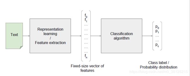
第一步：Representation learning/Feature extraction，其实词的one-hot向量直接相加就一种简单的Representation learning，向量中没有包含上下文关系、词和词之间没有联系和向量维度过大都是缺点。

第二步：将特征向量丢给分类模型获得结果，https://blog.csdn.net/m0_38126215/article/details/84567473本文中就介绍了怎么使用朴素贝叶斯进行文本分类

2.CNN进行文本分类

下图就是一个简单的CNN模型，让我们来一步一步分析

第一层输入层：shape(词向量的维度，文本的长度)。词向量的维度是由你训练的词嵌入模型决定的，而文本长度可以是当前最长文本的长度，你也可以自己定一个。

卷积层：shape(词向量的维度，kernel_size)。上图的size是2，只挨个对上下两个词进行卷积操作，你可以可以选择3。当你选择的size大于2以后，你又要多考虑一个参数卷积右移时候的步长。

a. 举个例子解释卷积操作，用卷积操作结果为，一个序列是共享一个卷积神经的参数的，这样训练的过程就会减少很多工作量

b. 既然参数是共享的，那么一个convolution并不能提取多少有用的信息，所以图里用了32个卷积，所以图中维度写的是32*(100*2),当然你可以用64,128.

c. 衍生知识点 padding填充，无论是卷积的大小步长怎么选，你结果的向量的长度会比输入向量的长度要短，比如图中的9变成了8，padding就是在输入向量的前后填充一些0，保证输出的结果长度是你想要的！！如果你的文本的开头词和结束词非常重要，那么padding就是一个不错的选择，可以卷积充分的提取开头和结束词的信息（单纯自己的理解，没试验过，不喜勿喷）

第二层卷积后的输出：shape(卷积的数量，根据步长和卷积的size决定)

池化层：用于信息压缩，既然每个卷积神经提取的信息是有限的，那就有必要对每个卷积神经的结果一下池化一下。课上文本分析建议使用MAX的赤化方法。以图为例，每个卷积的结果是8个，我们只取8个中最大的一个。当然还有其他的池化方法，比如求平均数等等

第三层池化后的输出：shape(卷积的数量，1)，这时候的结果已经可以扔给线性模型去做分类了。

 

3.CNN文本分类提升

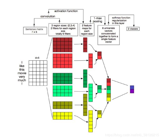
使用不同size的卷积神经对数据进行处理，如图所示

分别使用了sizes为2,3,4的卷积神经对数据进行操作，对卷积后的数据池化，接着讲池化后的数据concatenate到一起

二 Kaggle—工资预测

数据我放在网盘了https://pan.baidu.com/s/176lVyqWdFTpP8ydyB7c6NA，当然大家可以去比赛的页面观看工资预测页面

第一步 导入数据

import numpy as np
import pandas as pd
import matplotlib.pyplot as plt
%matplotlib inline
data = pd.read_csv(r"C:\Users\BF\Desktop\机器学习\nlp_course-master\Train_rev1.csv", index_col=None)
data.shape
print(data.head())

包含了如下数据

['Id', 'Title', 'FullDescription', 'LocationRaw', 'LocationNormalized', 'ContractType', 'ContractTime', 'Company', 'Category', 'SalaryRaw', 'SalaryNormalized', 'SourceName']

其中SalaryNormalized就是带预测的工资数据，是SalaryRaw的中位数。招聘信息中还包含了职位Title，详细描述，工作地点，合同类型，合同时间，岗位类别，公司的信息。其中【职位Title，详细描述】需要用到文本分析，而其他特征都可以转为01的特征向量。

第二步 查看数据

正常拿到数据的第一步是查看数据的的具体信息，分布图、箱线图和一般的统计描述等等。去除异常值、补全空值等等操作也是必要的。这里我们单纯的看一下收入的分布图，发现分布有偏我们log一下，然后将空值补NaN。

plt.figure(figsize=[8, 4])
plt.subplot(1, 2, 1)
plt.hist(data["SalaryNormalized"], bins=20);


data['Log1pSalary'] = np.log1p(data['SalaryNormalized']).astype('float32')  # 将工资数据log，使其变为正态分布

plt.subplot(1, 2, 2)
plt.hist(data['Log1pSalary'], bins=20);


text_columns = ["Title", "FullDescription"]
categorical_columns = ["Category", "Company", "LocationNormalized", "ContractType", "ContractTime"]
target_column = "Log1pSalary"

data[categorical_columns] = data[categorical_columns].fillna('NaN') # cast missing values to string "NaN"

第三步 准备一个word2vec模型

导入一个训练好的word2vec模型，使用此模型生成一个字典用于存储每个词的index——word2idx，接着生成一个矩阵将每个词对应的词向量放入其中——embeddings_matrix。

import gensim.downloader as api
wordmodel = api.load('glove-twitter-100')

#UNK和PAD是用处理没有遇见过的词和padding的时候用的
UNK, PAD = "UNK", "PAD"
word2idx = { } 
word2idx[UNK] = 0
word2idx[PAD] = 1  # 初始化 `[word : token]` 字典，后期 tokenize 语料库就是用该词典。
vocab_list = [(k, wordmodel.wv[k]) for k, v in wordmodel.wv.vocab.items()]

# 存储所有 word2vec 中所有向量的数组
embeddings_matrix = np.zeros((len(wordmodel.wv.vocab.items()) + 2, wordmodel.vector_size))
print('Found %s word vectors.' % len(wordmodel.wv.vocab.items()))
for i in range(len(vocab_list)):
    word = vocab_list[i][0]
    word2idx[word] = i + 2
    embeddings_matrix[i + 2] = vocab_list[i][1]

第四步 使用word2idx将文本转向量

UNK_IX, PAD_IX = map(word2idx.get, [UNK, PAD])
print(UNK_IX, PAD_IX)
def as_matrix(sequences, max_len=None):
    
    if isinstance(sequences[0], str):  # 将str的数据类型转为 list
        sequences = list(map(str.split, sequences))

    # 矩阵的长度，当前文本的最大长度或者设置的max_len    
    max_len = min(max(map(len, sequences)), max_len or float('inf'))
    
    # 生成一个由PAD_IX填充的矩阵
    matrix = np.full((len(sequences), max_len), np.int32(PAD_IX))
    for i,seq in enumerate(sequences):
        # 遇到没见过的词使用UNK_IX
        row_ix = [word2idx.get(word, UNK_IX) for word in seq[:max_len]]
        matrix[i, :len(row_ix)] = row_ix
    
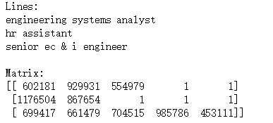
    return matrix

让我们来看看as_matrix的结果

print("Lines:")
print('\n'.join(data["Title"][::100000].values), end='\n\n')
print("Matrix:")
print(as_matrix(data["Title"][::100000]))

词已经变成了index，长度也统一了。

第五步 处理文本以外的特征

categorical_columns = ["Category", "Company", "LocationNormalized", "ContractType", "ContractTime"]，由于本文的重点是文本分析，所以其他的特征我们都简单转为01就好。举个例子把以公司为例

公司		腾讯	百度	阿里
腾讯		1	0	0
百度		0	1	0
阿里		0	0	1

 

Company字段包含的公司太多了，所以我们只取出现次数最多的1000个

from sklearn.feature_extraction import DictVectorizer
from collections import Counter
# we only consider top-1k most frequent companies to minimize memory usage
top_companies, top_counts = zip(*Counter(data['Company']).most_common(1000))
recognized_companies = set(top_companies)
data["Company"] = data["Company"].apply(lambda comp: comp if comp in recognized_companies else "Other")

categorical_vectorizer = DictVectorizer(dtype=np.float32, sparse=False)
categorical_vectorizer.fit(data[categorical_columns].apply(dict, axis=1))

第六步 为CNN准备数据

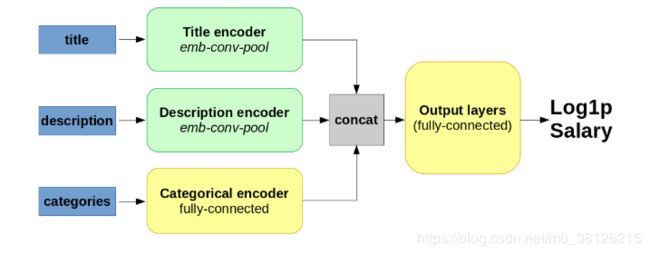
首先介绍一下一下本次要搭建的结构，分别对title 和 description进行卷积操作（包含词嵌入，卷积和池化），对其他categories直接全连接（简单理解成线性+激活函数）

由于我们的的input是3块，所以我们需要一个字典分别存储三块数据

from sklearn.model_selection import train_test_split
# 将数据切为训练集和开发集，开发集的作用我前面的文章介绍过
data_train, data_val = train_test_split(data, test_size=0.2, random_state=42)
data_train.index = range(len(data_train))
data_val.index = range(len(data_val))

print("Train size = ", len(data_train))
print("Validation size = ", len(data_val))

def make_batch(data, max_len=None, word_dropout=0):
    """
    Creates a keras-friendly dict from the batch data.
    :param word_dropout: replaces token index with UNK_IX with this probability
    :returns: a dict with {'title' : int64[batch, title_max_len]
    """
    #调用as_matrix方法处理数据
    batch = {}
    batch["Title"] = as_matrix(data["Title"].values, max_len)
    batch["FullDescription"] = as_matrix(data["FullDescription"].values, max_len)
    batch['Categorical'] = categorical_vectorizer.transform(data[categorical_columns].apply(dict, axis=1))
    
    #word_dropout参数用于控制
    if word_dropout != 0:
        batch["FullDescription"] = apply_word_dropout(batch["FullDescription"], 1. - word_dropout)
    
    # 将目标Log1pSalary字段取出
    if target_column in data.columns:
        batch[target_column] = data[target_column].values
    
    return batch


def apply_word_dropout(matrix, keep_prop, replace_with=UNK_IX, pad_ix=PAD_IX,):
    # 根据概率生成一个01矩阵
    # 2代表range(2),生成的数字只能是0,1。np.shape(matrix)代表最终生成矩阵的大小。p代表01分别的概率
    dropout_mask = np.random.choice(2, np.shape(matrix), p=[keep_prop, 1 - keep_prop]) 

    #保证dropout_mask只对非填充列进行操作
    dropout_mask &= matrix != pad_ix
    
    # np.full_like(matrix, replace_with)生成全0的矩阵
    # 使用np.choose 根据dropout_mask 来挑选是用matrix还是用0
    # 其实这里可以用矩阵的点乘进行，不用这么复杂
    return np.choose(dropout_mask, [matrix, np.full_like(matrix, replace_with)]) 

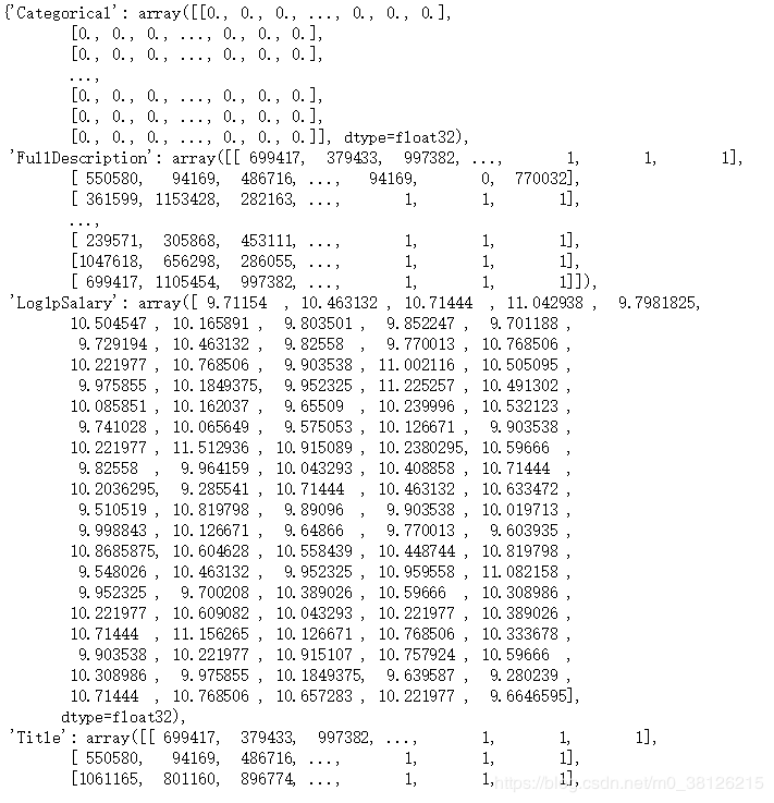
print(make_batch(data_train[:100]))

来看看结果

第七步 搭建CNN

踩坑总结

1. cnn的输入是词的index序列！！

2. 卷积神经使用L.Conv1D，Conv2D应该是在图像处理中使用的！！

3 激活函数的选择！！我们最终预测的数是log1salary，这个值的大小在10左右。刚开始我output_layer选择的Tanh作为激活函数，tanh的输出是-1到1之间的，所以永远别想得到正确的结果。激活函数的选择非常重要！

import keras
import keras.layers as L


def build_model(n_tokens=len(embeddings_matrix), n_cat_features=len(categorical_vectorizer.vocabulary_), hid_size=32):
    """ Build a model that maps three data sources to a single linear output: predicted log1p(salary) """

    # 确定数据，我们input的数据其实是字典，所有通过Input来从字典中分别导入数据
    l_title = L.Input(shape=[None], name="Title") 
    l_descr = L.Input(shape=[None], name="FullDescription")
    l_categ = L.Input(shape=[n_cat_features], name="Categorical")
    
    
    # #Embedding Layer 是针对NLP的，将原始One-Hot编码的词（长度为词库大小）映射到低维向量表达，降低特征维数，我们可以把我们训练的word2vec放入其中。

    l_title_emb = L.Embedding(output_dim=100, input_dim=n_tokens, input_length=100, weights=[embeddings_matrix], trainable=False)(l_title) 
    l_descr_emb = L.Embedding(output_dim=100, input_dim=n_tokens, input_length=1000, weights=[embeddings_matrix], trainable=False)(l_descr)
    l_categ_ful = L.Dense(hid_size, activation='relu')(l_categ)

    
    filters = hid_size
    fsz = 3
    l_title_conv1 = L.Conv1D(filters,kernel_size=fsz,activation='relu')(l_title_emb)
    l_descr_conv1 = L.Conv1D(filters,kernel_size=fsz,activation='relu')(l_descr_emb)
    l_title_pool1= L.GlobalMaxPooling1D()(l_title_conv1)
    l_descr_pool1= L.GlobalMaxPooling1D()(l_descr_conv1)
    
    concat = keras.layers.concatenate([l_title_pool1, l_descr_pool1, l_categ_ful])
    

    output_layer = L.Dense(1, activation='relu' , name='log1salary')(concat)

    
    model = keras.models.Model(inputs=[l_title, l_descr, l_categ], outputs=[output_layer])

    #模型使用adam的优化方法，lossfunction使用mean_squared_error
    model.compile('adam', 'mean_squared_error', metrics=['mean_absolute_error'])
    return model

model = build_model()
model.summary()

此时你就可以通过summary查看你搭建的CNN的具体信息了

第八步 开始训练

 

# 这是一个迭代器，给模型input size为batch_size=的数据
def iterate_minibatches(data, batch_size=256, shuffle=True, cycle=False, **kwargs):
    """ iterates minibatches of data in random order """
    while True:
        indices = np.arange(len(data))
        if shuffle:
            indices = np.random.permutation(indices)

        for start in range(0, len(indices), batch_size):
            batch = make_batch(data.iloc[indices[start : start + batch_size]], **kwargs)
            target = batch.pop(target_column)
            yield batch, target
        
        if not cycle: break



batch_size = 256
epochs = 30           # definitely too small
steps_per_epoch = 100  # for full pass over data: (len(data_train) - 1) // batch_size + 1

model = build_model()

model.fit_generator(iterate_minibatches(data_train, batch_size, cycle=True, word_dropout=0.05), 
                    epochs=epochs, steps_per_epoch=steps_per_epoch,
                    
                    validation_data=iterate_minibatches(data_val, batch_size, cycle=True), # 设置验证集
                    validation_steps=data_val.shape[0] // batch_size
                   )

epochs  = 30 进行训练结果如下，可以发现lossfunction已经很小了，但是我们预测是Log1pSalary别忘了，任何一点小的差异在还原为Salary后就会差很多了！所以建议增加训练次数，或者更改模型结构。

Epoch 1/30
100/100 [==============================] - 84s 840ms/step - loss: 8.2737 - mean_absolute_error: 1.8540 - val_loss: 0.8820 - val_mean_absolute_error: 0.7357
Epoch 11/30
100/100 [==============================] - 83s 826ms/step - loss: 0.1646 - mean_absolute_error: 0.3108 - val_loss: 0.1571 - val_mean_absolute_error: 0.3055
Epoch 21/30
100/100 [==============================] - 84s 841ms/step - loss: 0.1174 - mean_absolute_error: 0.2600 - val_loss: 0.1114 - 
Epoch 30/30
100/100 [==============================] - 86s 859ms/step - loss: 0.0976 - mean_absolute_error: 0.2356 - val_loss: 0.0960 - val_mean_absolute_error: 0.2365

 

第九步 看看结果吧

随机选择开发集中的一个数据，查看预测结果

i = np.random.randint(len(data_val))
print("Index:", i)
print("Salary (gbp):", np.expm1(model.predict(make_batch(data_val.iloc[i: i+1]))[0, 0]))
print(data.iloc[i: i+1])