Coursera吴恩达机器学习课程 总结笔记及作业代码——第7周支持向量机
1.1 Optimization objective
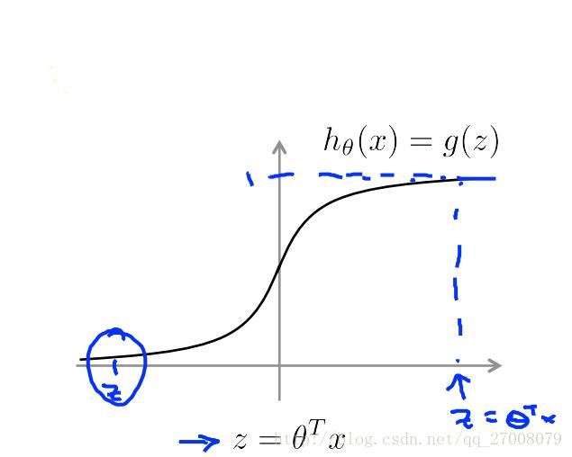
IF y=1, we want hθ(x)≈1 , θTx≫0
IF y=0, we want hθ(x)≈0 , θTx≪0
其CostFunction为:
J(θ)=1m[∑mi=1y(i)(−loghθ(x(i)))+(1−y(i))(−(log(1−hθ(x(i)))))]+λ2m∑mj=1θ2j
我们看下在SVM中对costfunction的改变
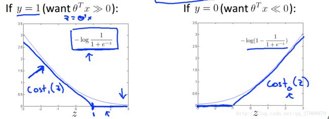
将其中log函数部分换成了蓝色折线所代表的cost函数。
costFunction也相应的改变为
J(θ)=1m[∑mi=1y(i)Cost1(θTx(i))+(1−y(i))Cost0(θTx(i))]+λ2m∑mj=1θ2j
在SVM中,我们常常用C代替 λ
J(θ)=C∑mi=1[y(i)Cost1(θTx(i))+(1−y(i))Cost0(θTx(i))]+12∑mj=1θ2j
1.2 Large Margin Intuition
IF y=1, we want θTx≥1 (not just ≥0 )
IF y=0, we want θTx≤−1 (not just ≤0 )
即min 12∑ni=1θ2j
θTx(i)≥+1 if y(i)=1
θTx(i)≤−1 if y(i)=0
归结起来为一个条件极值问题
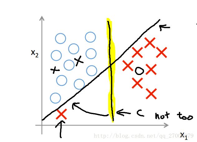
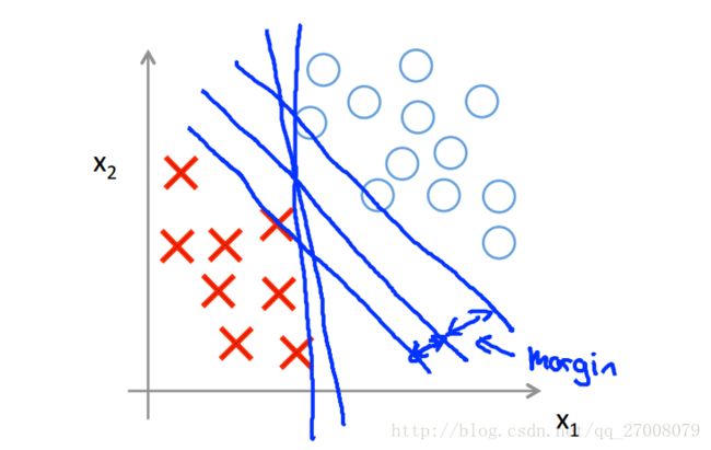
SVM通过寻找分类中淡黄色背景的那条线作为边界,而不是其余满足条件的边界,因此SVM又被称为大间隔分类器。
1.3 The mathematics behind large margin classification
下面我们从数学角度看一下SVM
通过简化问题,我们知道要求的最小值为 ||θ|| 的最小值,即 θ 的范数最小值

下面看一下限制条件代表的含义,通过高中数学,我们知道两个向量相乘的几何含义如下

通过上面可知,我们要求 ||θ|| 的最小值,因此我们希望 p(i) 尽量大。
假如选择了下面图中的绿色线作为边界,我们会发现 p(i) 比较小,这样不能得出 ||θ|| 的最小值
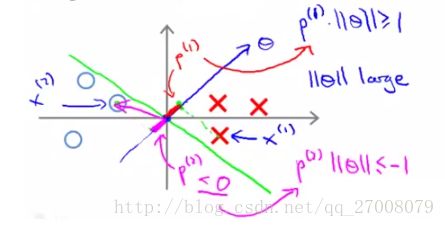
如果选择下面的绿色线作为边界,我们可以得到较小的 ||θ|| 值

这样我们就从直观上感受了SVM作为大间距分类器的效果。
1.4 Kernels
在这里我们通过引入核函数来解决这个问题。
假设函数 hθ(x)=θ0+θ1f1+θ2f2+θ3f3+⋯
给出几个向量 l(i) 作为landmarks
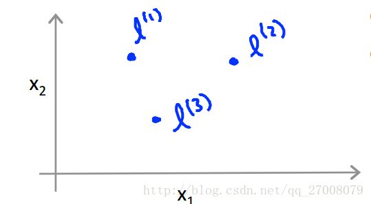
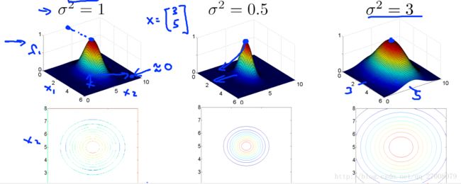
fi=similarity(x(i),l(i))=exp(−||x(i)−l(i)||22δ2)
exp中的函数为高斯核函数
If x(i)≈l(i)
fi≈exp(−022δ2)≈1
If x(i) is far from l(i)
fi≈exp(−(large number)22δ2)≈0
关于landmarks我们应该怎么选取呢?
我们可以把x个数据集作为landmarks

这样,对于每一个训练集中的数据,我们都有一个m+1维向量与之对应。

在预测时

关于参数对算法的影响
大C:低偏差,高方差(对应低 λ )
小C:高偏差,低方差(对应高 λ )
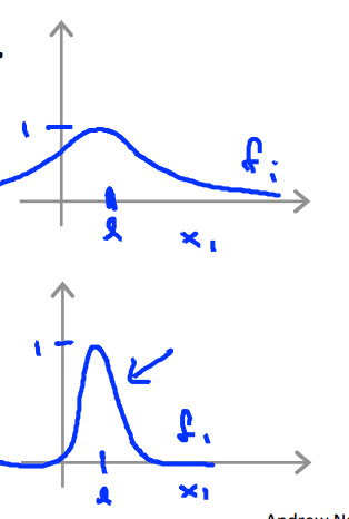
大 δ2 : fi 分布更平滑,高偏差,低方差
小 δ2 : fi 分布更集中,低偏差,高方差
2 程序代码
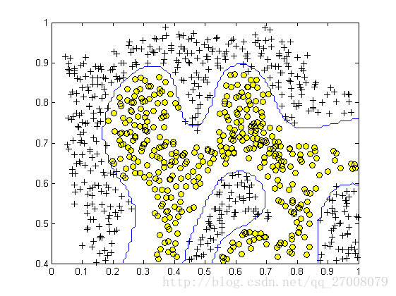
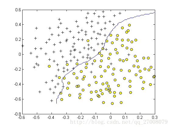
2.1 使用SVM构建分类器,进行非线性分类,最后选择不同的C值选出最好的边界线。
ex6.m
%% Machine Learning Online Class
%  Exercise 6 | Support Vector Machines
%
%  Instructions
%  ------------
%
%  This file contains code that helps you get started on the
%  exercise. You will need to complete the following functions:
%
%     gaussianKernel.m
%     dataset3Params.m
%     processEmail.m
%     emailFeatures.m
%
%  For this exercise, you will not need to change any code in this file,
%  or any other files other than those mentioned above.
%

%% Initialization
clear ; close all; clc

%% =============== Part 1: Loading and Visualizing Data ================
%  We start the exercise by first loading and visualizing the dataset.
%  The following code will load the dataset into your environment and plot
%  the data.
%

fprintf('Loading and Visualizing Data ...\n')

% Load from ex6data1:
% You will have X, y in your environment
load('ex6data1.mat');

% Plot training data
plotData(X, y);

fprintf('Program paused. Press enter to continue.\n');
pause;

%% ==================== Part 2: Training Linear SVM ====================
%  The following code will train a linear SVM on the dataset and plot the
%  decision boundary learned.
%

% Load from ex6data1:
% You will have X, y in your environment
load('ex6data1.mat');

fprintf('\nTraining Linear SVM ...\n')

% You should try to change the C value below and see how the decision
% boundary varies (e.g., try C = 1000)
C = 1;
model = svmTrain(X, y, C, @linearKernel, 1e-3, 20);
visualizeBoundaryLinear(X, y, model);

fprintf('Program paused. Press enter to continue.\n');
pause;

%% =============== Part 3: Implementing Gaussian Kernel ===============
%  You will now implement the Gaussian kernel to use
%  with the SVM. You should complete the code in gaussianKernel.m
%
fprintf('\nEvaluating the Gaussian Kernel ...\n')

x1 = [1 2 1]; x2 = [0 4 -1]; sigma = 2;
sim = gaussianKernel(x1, x2, sigma);

fprintf(['Gaussian Kernel between x1 = [1; 2; 1], x2 = [0; 4; -1], sigma = %f :' ...
         '\n\t%f\n(for sigma = 2, this value should be about 0.324652)\n'], sigma, sim);

fprintf('Program paused. Press enter to continue.\n');
pause;

%% =============== Part 4: Visualizing Dataset 2 ================
%  The following code will load the next dataset into your environment and
%  plot the data.
%

fprintf('Loading and Visualizing Data ...\n')

% Load from ex6data2:
% You will have X, y in your environment
load('ex6data2.mat');

% Plot training data
plotData(X, y);

fprintf('Program paused. Press enter to continue.\n');
pause;

%% ========== Part 5: Training SVM with RBF Kernel (Dataset 2) ==========
%  After you have implemented the kernel, we can now use it to train the
%  SVM classifier.
%
fprintf('\nTraining SVM with RBF Kernel (this may take 1 to 2 minutes) ...\n');

% Load from ex6data2:
% You will have X, y in your environment
load('ex6data2.mat');

% SVM Parameters
C = 1; sigma = 0.1;

% We set the tolerance and max_passes lower here so that the code will run
% faster. However, in practice, you will want to run the training to
% convergence.
model= svmTrain(X, y, C, @(x1, x2) gaussianKernel(x1, x2, sigma));
visualizeBoundary(X, y, model);

fprintf('Program paused. Press enter to continue.\n');
pause;

%% =============== Part 6: Visualizing Dataset 3 ================
%  The following code will load the next dataset into your environment and
%  plot the data.
%

fprintf('Loading and Visualizing Data ...\n')

% Load from ex6data3:
% You will have X, y in your environment
load('ex6data3.mat');

% Plot training data
plotData(X, y);

fprintf('Program paused. Press enter to continue.\n');
pause;

%% ========== Part 7: Training SVM with RBF Kernel (Dataset 3) ==========

%  This is a different dataset that you can use to experiment with. Try
%  different values of C and sigma here.
%

% Load from ex6data3:
% You will have X, y in your environment
load('ex6data3.mat');

% Try different SVM Parameters here
[C, sigma] = dataset3Params(X, y, Xval, yval);

% Train the SVM
model= svmTrain(X, y, C, @(x1, x2) gaussianKernel(x1, x2, sigma));
visualizeBoundary(X, y, model);

fprintf('Program paused. Press enter to continue.\n');
pause;
gaussianKernel.m
function sim = gaussianKernel(x1, x2, sigma)
%RBFKERNEL returns a radial basis function kernel between x1 and x2
%   sim = gaussianKernel(x1, x2) returns a gaussian kernel between x1 and x2
%   and returns the value in sim

% Ensure that x1 and x2 are column vectors
x1 = x1(:); x2 = x2(:);

% You need to return the following variables correctly.
sim = 0;

% ====================== YOUR CODE HERE ======================
% Instructions: Fill in this function to return the similarity between x1
%               and x2 computed using a Gaussian kernel with bandwidth
%               sigma
%
%

sim = exp(-sum((x1 - x2).^2)/2/sigma^2);

% =============================================================

end
dataset3Params.m
function [C, sigma] = dataset3Params(X, y, Xval, yval)
%DATASET3PARAMS returns your choice of C and sigma for Part 3 of the exercise
%where you select the optimal (C, sigma) learning parameters to use for SVM
%with RBF kernel
%   [C, sigma] = DATASET3PARAMS(X, y, Xval, yval) returns your choice of C and
%   sigma. You should complete this function to return the optimal C and
%   sigma based on a cross-validation set.
%

% You need to return the following variables correctly.
C = 1;
sigma = 0.3;

% ====================== YOUR CODE HERE ======================
% Instructions: Fill in this function to return the optimal C and sigma
%               learning parameters found using the cross validation set.
%               You can use svmPredict to predict the labels on the cross
%               validation set. For example,
%                   predictions = svmPredict(model, Xval);
%               will return the predictions on the cross validation set.
%
%  Note: You can compute the prediction error using
%        mean(double(predictions ~= yval))
%
cc = [0.01, 0.03, 0.1, 0.3, 1, 3, 10, 30];
ss = cc;
maxx = 0;

for i=1:length(cc)
    for j=1:length(cc)
        model = svmTrain(X, y, cc(i), @(x1, x2) gaussianKernel(x1, x2, ss(j)));
        predict = svmPredict(model, Xval);
        cur = mean(double(predict == yval));
        if maxx < cur
            maxx = cur;
            C = cc(i);
            sigma = ss(j);
        end
    end
end

% =========================================================================

end
2.2垃圾邮件分类器
ex6_spam.m
%% Machine Learning Online Class
%  Exercise 6 | Spam Classification with SVMs
%
%  Instructions
%  ------------
%
%  This file contains code that helps you get started on the
%  exercise. You will need to complete the following functions:
%
%     gaussianKernel.m
%     dataset3Params.m
%     processEmail.m
%     emailFeatures.m
%
%  For this exercise, you will not need to change any code in this file,
%  or any other files other than those mentioned above.
%

%% Initialization
clear ; close all; clc

%% ==================== Part 1: Email Preprocessing ====================
%  To use an SVM to classify emails into Spam v.s. Non-Spam, you first need
%  to convert each email into a vector of features. In this part, you will
%  implement the preprocessing steps for each email. You should
%  complete the code in processEmail.m to produce a word indices vector
%  for a given email.

fprintf('\nPreprocessing sample email (emailSample1.txt)\n');

% Extract Features
file_contents = readFile('emailSample1.txt');
word_indices  = processEmail(file_contents);

% Print Stats
fprintf('Word Indices: \n');
fprintf(' %d', word_indices);
fprintf('\n\n');

fprintf('Program paused. Press enter to continue.\n');
pause;

%% ==================== Part 2: Feature Extraction ====================
%  Now, you will convert each email into a vector of features in R^n.
%  You should complete the code in emailFeatures.m to produce a feature
%  vector for a given email.

fprintf('\nExtracting features from sample email (emailSample1.txt)\n');

% Extract Features
file_contents = readFile('emailSample1.txt');
word_indices  = processEmail(file_contents);
features      = emailFeatures(word_indices);

% Print Stats
fprintf('Length of feature vector: %d\n', length(features));
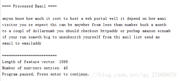
fprintf('Number of non-zero entries: %d\n', sum(features > 0));

fprintf('Program paused. Press enter to continue.\n');
pause;

%% =========== Part 3: Train Linear SVM for Spam Classification ========
%  In this section, you will train a linear classifier to determine if an
%  email is Spam or Not-Spam.

% Load the Spam Email dataset
% You will have X, y in your environment
load('spamTrain.mat');

fprintf('\nTraining Linear SVM (Spam Classification)\n')
fprintf('(this may take 1 to 2 minutes) ...\n')

C = 0.1;
model = svmTrain(X, y, C, @linearKernel);

p = svmPredict(model, X);

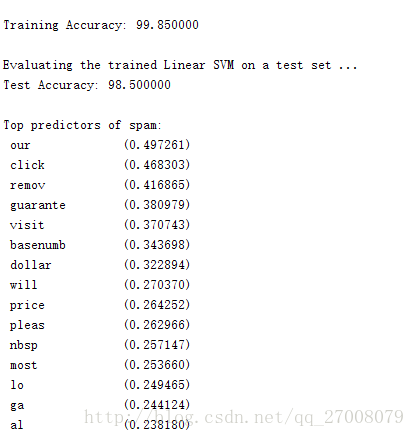
fprintf('Training Accuracy: %f\n', mean(double(p == y)) * 100);

%% =================== Part 4: Test Spam Classification ================
%  After training the classifier, we can evaluate it on a test set. We have
%  included a test set in spamTest.mat

% Load the test dataset
% You will have Xtest, ytest in your environment
load('spamTest.mat');

fprintf('\nEvaluating the trained Linear SVM on a test set ...\n')

p = svmPredict(model, Xtest);

fprintf('Test Accuracy: %f\n', mean(double(p == ytest)) * 100);
pause;


%% ================= Part 5: Top Predictors of Spam ====================
%  Since the model we are training is a linear SVM, we can inspect the
%  weights learned by the model to understand better how it is determining
%  whether an email is spam or not. The following code finds the words with
%  the highest weights in the classifier. Informally, the classifier
%  'thinks' that these words are the most likely indicators of spam.
%

% Sort the weights and obtin the vocabulary list
[weight, idx] = sort(model.w, 'descend');
vocabList = getVocabList();

fprintf('\nTop predictors of spam: \n');
for i = 1:15
    fprintf(' %-15s (%f) \n', vocabList{idx(i)}, weight(i));
end

fprintf('\n\n');
fprintf('\nProgram paused. Press enter to continue.\n');
pause;

%% =================== Part 6: Try Your Own Emails =====================
%  Now that you've trained the spam classifier, you can use it on your own
%  emails! In the starter code, we have included spamSample1.txt,
%  spamSample2.txt, emailSample1.txt and emailSample2.txt as examples.
%  The following code reads in one of these emails and then uses your
%  learned SVM classifier to determine whether the email is Spam or
%  Not Spam

% Set the file to be read in (change this to spamSample2.txt,
% emailSample1.txt or emailSample2.txt to see different predictions on
% different emails types). Try your own emails as well!
filename = 'spamSample1.txt';

% Read and predict
file_contents = readFile(filename);
word_indices  = processEmail(file_contents);
x             = emailFeatures(word_indices);
p = svmPredict(model, x);

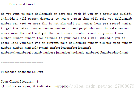
fprintf('\nProcessed %s\n\nSpam Classification: %d\n', filename, p);
fprintf('(1 indicates spam, 0 indicates not spam)\n\n');
processEmail.m
function word_indices = processEmail(email_contents)
%PROCESSEMAIL preprocesses a the body of an email and
%returns a list of word_indices
%   word_indices = PROCESSEMAIL(email_contents) preprocesses
%   the body of an email and returns a list of indices of the
%   words contained in the email.
%

% Load Vocabulary
vocabList = getVocabList();

% Init return value
word_indices = [];

% ========================== Preprocess Email ===========================

% Find the Headers ( \n\n and remove )
% Uncomment the following lines if you are working with raw emails with the
% full headers

% hdrstart = strfind(email_contents, ([char(10) char(10)]));
% email_contents = email_contents(hdrstart(1):end);

% Lower case
email_contents = lower(email_contents);

% Strip all HTML
% Looks for any expression that starts with < and ends with > and replace
% and does not have any < or > in the tag it with a space
email_contents = regexprep(email_contents, '<[^<>]+>', ' ');

% Handle Numbers
% Look for one or more characters between 0-9
email_contents = regexprep(email_contents, '[0-9]+', 'number');

% Handle URLS
% Look for strings starting with http:// or https://
email_contents = regexprep(email_contents, ...
                           '(http|https)://[^\s]*', 'httpaddr');

% Handle Email Addresses
% Look for strings with @ in the middle
email_contents = regexprep(email_contents, '[^\s]+@[^\s]+', 'emailaddr');

% Handle $ sign
email_contents = regexprep(email_contents, '[$]+', 'dollar');


% ========================== Tokenize Email ===========================

% Output the email to screen as well
fprintf('\n==== Processed Email ====\n\n');

% Process file
l = 0;

while ~isempty(email_contents)

    % Tokenize and also get rid of any punctuation
    [str, email_contents] = ...
       strtok(email_contents, ...
              [' @$/#.-:&*+=[]?!(){},''">_<;%' char(10) char(13)]);

    % Remove any non alphanumeric characters
    str = regexprep(str, '[^a-zA-Z0-9]', '');

    % Stem the word
    % (the porterStemmer sometimes has issues, so we use a try catch block)
    try str = porterStemmer(strtrim(str));
    catch str = ''; continue;
    end;

    % Skip the word if it is too short
    if length(str) < 1
       continue;
    end

    % Look up the word in the dictionary and add to word_indices if
    % found
    % ====================== YOUR CODE HERE ======================
    % Instructions: Fill in this function to add the index of str to
    %               word_indices if it is in the vocabulary. At this point
    %               of the code, you have a stemmed word from the email in
    %               the variable str. You should look up str in the
    %               vocabulary list (vocabList). If a match exists, you
    %               should add the index of the word to the word_indices
    %               vector. Concretely, if str = 'action', then you should
    %               look up the vocabulary list to find where in vocabList
    %               'action' appears. For example, if vocabList{18} =
    %               'action', then, you should add 18 to the word_indices
    %               vector (e.g., word_indices = [word_indices ; 18]; ).
    %
    % Note: vocabList{idx} returns a the word with index idx in the
    %       vocabulary list.
    %
    % Note: You can use strcmp(str1, str2) to compare two strings (str1 and
    %       str2). It will return 1 only if the two strings are equivalent.
    %
    for i=1:length(vocabList)
        if strcmp(vocabList{i}, str)
            word_indices = [word_indices; i];
            break;
        end
    end

    % =============================================================


    % Print to screen, ensuring that the output lines are not too long
    if (l + length(str) + 1) > 78
        fprintf('\n');
        l = 0;
    end
    fprintf('%s ', str);
    l = l + length(str) + 1;

end

% Print footer
fprintf('\n\n=========================\n');

end
emailFeatures.m
function x = emailFeatures(word_indices)
%EMAILFEATURES takes in a word_indices vector and produces a feature vector
%from the word indices
%   x = EMAILFEATURES(word_indices) takes in a word_indices vector and
%   produces a feature vector from the word indices.

% Total number of words in the dictionary
n = 1899;

% You need to return the following variables correctly.
x = zeros(n, 1);

% ====================== YOUR CODE HERE ======================
% Instructions: Fill in this function to return a feature vector for the
%               given email (word_indices). To help make it easier to
%               process the emails, we have have already pre-processed each
%               email and converted each word in the email into an index in
%               a fixed dictionary (of 1899 words). The variable
%               word_indices contains the list of indices of the words
%               which occur in one email.
%
%               Concretely, if an email has the text:
%
%                  The quick brown fox jumped over the lazy dog.
%
%               Then, the word_indices vector for this text might look
%               like:
%
%                   60  100   33   44   10     53  60  58   5
%
%               where, we have mapped each word onto a number, for example:
%
%                   the   -- 60
%                   quick -- 100
%                   ...
%
%              (note: the above numbers are just an example and are not the
%               actual mappings).
%
%              Your task is take one such word_indices vector and construct
%              a binary feature vector that indicates whether a particular
%              word occurs in the email. That is, x(i) = 1 when word i
%              is present in the email. Concretely, if the word 'the' (say,
%              index 60) appears in the email, then x(60) = 1. The feature
%              vector should look like:
%
%              x = [ 0 0 0 0 1 0 0 0 ... 0 0 0 0 1 ... 0 0 0 1 0 ..];
%
%
for i=1:length(word_indices)
    x(word_indices(i)) = 1;
end

% =========================================================================


end
