《统计学习方法》第二章 感知机 Perceptron 总结及其代码实现
文章中代码来自:https://github.com/wzyonggege/statistical-learning-method
看过SVM支持向量机的人应该对感知机很熟悉,感知机是一个线性分类器,是向量机的基础。
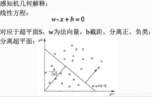
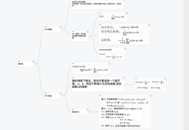
感知机(perceptron)是二类分类的线性分类模型,其输入为实例的特征向量,输出 为实例的类别,取+1和–1二值。感知机对应于输入空间(特征空间)中将实例划分为正 负两类的分离超平面,属于判别模型。感知机学习旨在求出将训练数据进行线性划分的分 离超平面,为此,导入基于误分类的损失函数,利用梯度下降法对损失函数进行极小化, 求得感知机模型。感知机学习算法具有简单而易于实现的优点,分为原始形式和对偶形 式。感知机预测是用学习得到的感知机模型对新的输入实例进行分类。
所以说,感知机能将线性可分的数据集分开。这意味着在二维平面上可以用一条线将正负样本分开,在三维空间中用一个平面将正负样本分开。
定义(感知机):
假设输入空间(特征空间)是![]() 输出空间是
输出空间是![]()
输入 ![]() 表示实例的特征向量,对应于输入空间(特 征空间)的点,输出
表示实例的特征向量,对应于输入空间(特 征空间)的点,输出 ![]() 表示实例的类别,由输入空 间到输出空间的函数:
表示实例的类别,由输入空 间到输出空间的函数:
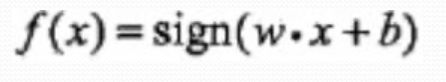
称为感知机,
模型参数:w x,内积,权值向量,偏置, 符号函数: 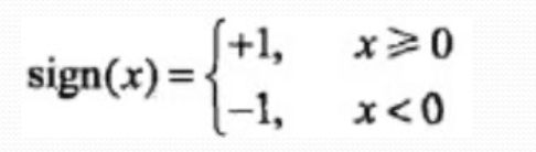
接下来是感知机的代码实现
import pandas as pd
import numpy as np
from sklearn.datasets import load_iris
import matplotlib.pyplot as plt
# load data
iris = load_iris()
df = pd.DataFrame(iris.data, columns=iris.feature_names) #将列名设置为特征
df['label'] = iris.target #增加一列为类别标签
#print(df.columns)
#将各个列重命名
df.columns = ['sepal length', 'sepal width', 'petal length', 'petal width', 'label']
df.label.value_counts() #value_counts确认数据出现的频率
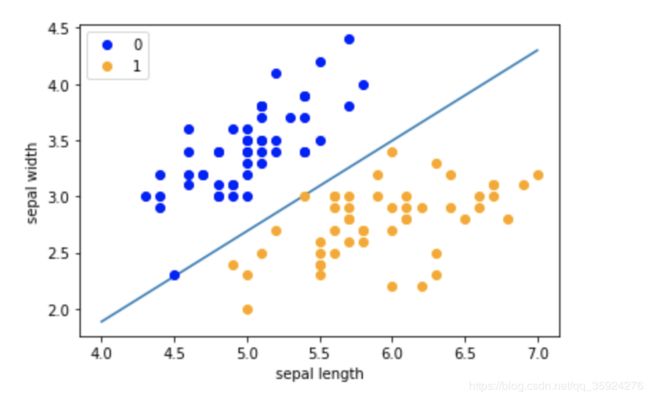
#绘制散点图
plt.scatter(df[:50]['sepal length'], df[:50]['sepal width'], label='0')
plt.scatter(df[50:100]['sepal length'], df[50:100]['sepal width'], label='1')
plt.xlabel('sepal length')
plt.ylabel('sepal width')
plt.legend() #给图加上图例
plt.show()
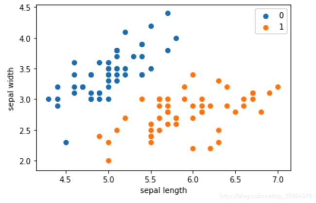
首先将数据集中的点都打印出来,我们可以看到这些数据按照类别是线形可分的。
接下来我们按照书中的算法构造分类器。
import pandas as pd
import numpy as np
from sklearn.datasets import load_iris
import matplotlib.pyplot as plt

# load data
iris = load_iris()
df = pd.DataFrame(iris.data, columns=iris.feature_names) #将列名设置为特征
df['label'] = iris.target         #增加一列为类别标签
#print(df.columns)

#将各个列重命名
df.columns = ['sepal length', 'sepal width', 'petal length', 'petal width', 'label']
df.label.value_counts() #value_counts确认数据出现的频率

data = np.array(df.iloc[:100, [0, 1, -1]])  #按行索引,取出第0,1,-1列
X, y = data[:,:-1], data[:,-1] #X为sepal length,sepal width y为标签
y = np.array([1 if i == 1 else -1 for i in y]) #将两个类别设重新设置为+1  —1
# 数据线性可分,二分类数据
# 此处为一元一次线性方程
class Model:
    def __init__(self):
        #将参数w1,w2置为1 b置为0 学习率为0.1
        self.w = np.ones(len(data[0])-1, dtype=np.float32)  #data[0]为第一行的数据len(data[0]=3)这里取两个w权重参数
        self.b = 0
        self.l_rate = 0.1
        # self.data = data

    def sign(self, x, w, b):
        y = np.dot(x, w) + b
        return y

    # 随机梯度下降法
    def fit(self, X_train, y_train):
        is_wrong = False#判断是否误分类
        while not is_wrong:
            wrong_count = 0
            for d in range(len(X_train)):
                #取出样例
                X = X_train[d]
                y = y_train[d]
                    #该点是误分类点,所以需要更新参数
                if y * self.sign(X, self.w, self.b) <= 0:
                    self.w = self.w + self.l_rate*np.dot(y, X)
                    self.b = self.b + self.l_rate*y
                    wrong_count += 1
            if wrong_count == 0:    #直到误分类点为0 跳出循环
                is_wrong = True
        return 'Perceptron Model!'

    #源代码中没有实现score的部分参考网上其他的一些补充了这一部分
    def predict(self, X):
        y = np.dot(X,self.w) + self.b
        return 1 if y >0 else -1
    def score(self,X_test,y_test):#评价模型性能
        count = 0       #计算预测对的点的个数
        for d in range(len((X_test))):
            x = X_test[d]
            y = y_test[d]
            if y == self.predict(X):
                count += 1

        return count/len(X_test)
perceptron = Model()
perceptron.fit(X, y)
print(perceptron.w)    #打印参数w
# print(data[0])
x_points = np.linspace(4, 7,10)
y_ = -(perceptron.w[0]*x_points + perceptron.b)/perceptron.w[1]
plt.plot(x_points, y_)

plt.plot(data[:50, 0], data[:50, 1], 'bo', color='blue', label='0')
plt.plot(data[50:100, 0], data[50:100, 1], 'bo', color='orange', label='1')
plt.xlabel('sepal length')
plt.ylabel('sepal width')
plt.legend()
plt.show()
可以得到这个图。
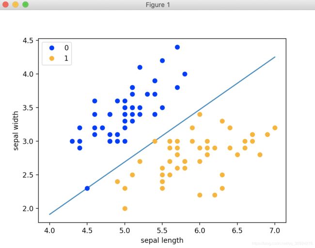
接下来的示例是使用sklearnzh 中感知机Perceptron实现。sklearn中都包装好了只需要输入一些参数即可。
import pandas as pd
import numpy as np
from sklearn.datasets import load_iris
import matplotlib.pyplot as plt

# load data
iris = load_iris()
df = pd.DataFrame(iris.data, columns=iris.feature_names) #将列名设置为特征
df['label'] = iris.target         #增加一列为类别标签
print(df.columns)
#将各个列重命名
df.columns = ['sepal length', 'sepal width', 'petal length', 'petal width', 'label']
df.label.value_counts() #value_counts确认数据出现的频率
data = np.array(df.iloc[:100, [0, 1, -1]])  #按行索引,取出第0,1,-1列
X, y = data[:,:-1], data[:,-1] #X为sepal length,sepal width y为标签  = np.array(df.iloc[:100, [0, 1, -1]])  #按行索引,取出第0,1,-1列
y = np.array([1 if i == 1 else -1 for i in y]) #将两个类别设重新设置为+1  —1
from sklearn.linear_model import Perceptron
#定义感知机
clf = Perceptron(fit_intercept=True, max_iter=1000, shuffle=True)
#使用训练数据拟合
clf.fit(X, y)
# Weights assigned to the features.得到训练结果,权重矩阵
print(clf.coef_)
# 超平面的截距 Constants in decision function.
print(clf.intercept_)
x_ponits = np.arange(4, 8)
y_ = -(clf.coef_[0][0]*x_ponits + clf.intercept_)/clf.coef_[0][1]
plt.plot(x_ponits, y_)

plt.plot(data[:50, 0], data[:50, 1], 'bo', color='blue', label='0')
plt.plot(data[50:100, 0], data[50:100, 1], 'bo', color='orange', label='1')
plt.xlabel('sepal length')
plt.ylabel('sepal width')
plt.legend()
plt.show()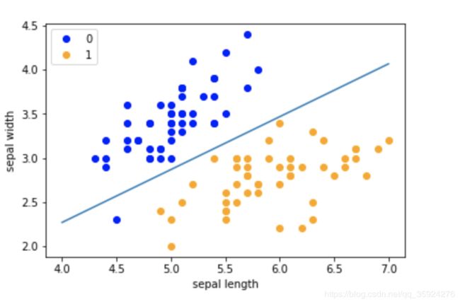
此时注意,上述结果图中还有一个蓝色点没有被分类正确。这是因为在SklearndePerceptron实例中有一个tol参数。
tol参数规定了如果本次迭代的损失和上次迭代的损失之差小于一个特定值时,停止迭代。所以我们需要设置tol=None 使之可以继续迭代:
上述的改为:
clf = Perceptron(fit_intercept=True, max_iter=1000,tol = None, shuffle=True)