Since we have learned some Random Walk theory in Statistical Physics, I chose this Chapter for my final project.
Random Walk
Abstract
In this project, I use the Random number generator for simulating the random walk.Every random system has a complicated trajectory, and it can be seen as a typical "Random Walk" in every direction. This is a progress in which "a walker" moves one step or none at a time.Hence, we can use this simple model to higher-dimension random system, such as diffusion.
Background
A random walk is a mathematical object which describes a path that consists of a succession of random steps. For example, the path traced by a molecule as it travels in a liquid or a gas, the search path of a foraging animal, superstring behavior, the price of a fluctuating stock and the financial status of a gambler can all be approximated by random walk models, even though they may not be truly random in reality. Random walks explain the observed behaviors of many processes in these fields, and thus serve as a fundamental model for the recorded stochastic activity.
Main Body
Diffusion is the net movement of molecules or atoms from a region of high concentration (or high chemical potential) to a region of low concentration (or low chemical potential).
1 Simple random walk
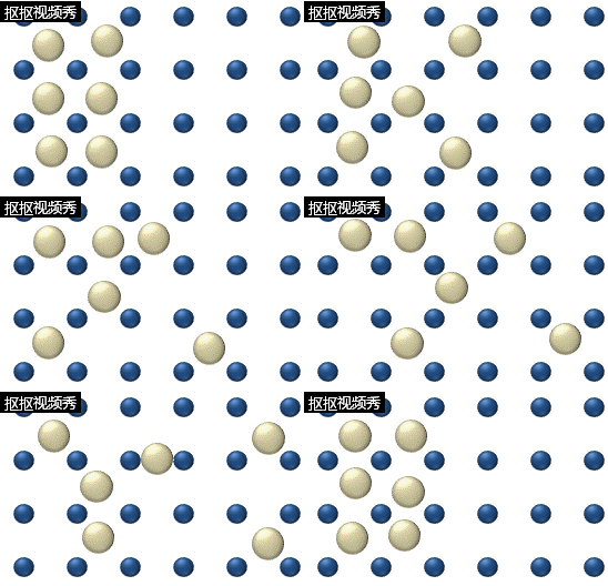
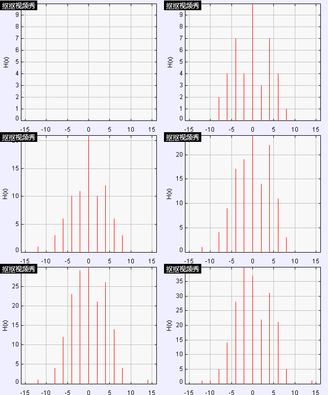
The simplest situation involves a walker that is able to take steps of length unity along a line. With the same probability of 1/2, we can see the distance will stay around 0 as thefigure shows .below.
Here is the code
Actually, since the random number is not always the same, we can get a little difference in twice simulation.That's the fluctuation in statistical physics.
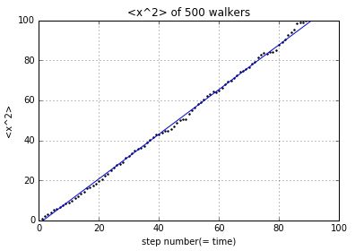
In diffusion situation, there is an interesting and informative quantity is
where t is the time, which here is just equal to the step number; and D is known as the diffusion constant.The simulation below can show the linear relation between
Here is the code
2 Typical example:Diffusion
As we metioned, random walks are equivalent to diffusion.We have
In one dimensional situation, we can approach this function as
Then we can set the initial parameters and use the progressive relationship to simulate the relation between density and time.
Here is the code
In the gif,we can see the every step change.
After the process, we can set the time to get a final result/
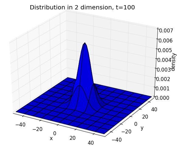
and we can see it in the three dimensional way
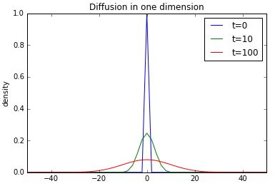
Actually, the density follows the function
where the "sigma" is "time" dependent It's a kind of Gaussian distribution, the simulation is corresponding with this function. We can see that when time becomes longer the curve will become wider and placid. That's consistent with theoretical situation.
Additional: entropy
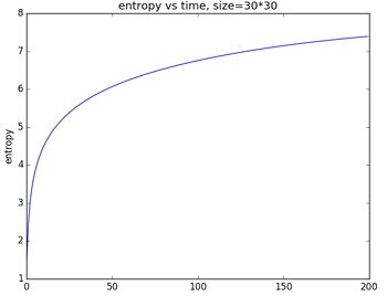
When a sugar resolves in a cup of water, we can see the diffusion process as a random phenomena.
As we can see, when time increases, the entropy value increases, but its growth speed is reduced. Eventually it will converge to a constant value.
Conclusion
For such equal possibility random walk, through simulation, we can find that the averange of a random behavior is around zero.And the square of x is linear to t with equal probability.
About the relationship between density and time, when time becomes longer the curve will become wider and placid.
As for entropy, the the entropy value increases, but its growth speed is reduced. Eventually it will converge to a constant value.
Acknowledgement
python画三维图的方法
matplotlib使用教程、和用python画动图的animation
制作GIF的抠抠视频秀
热统教材 statistical and thermal physics 以及本课程教材 computational physics
非常感谢蔡老师这种网络共享的作业方式,我作为一个基本不会编程语言的学生,通过一学期的学习和观看借鉴其他同学的代码,应该算对python这种语言初步有了了解,希望这种方式可以一直延续下去。

