注,有疑问 加QQ群..[174225475].. 共同探讨进步
有偿求助请 出门左转 door , 合作愉快
原理概念描述
案例:
有10000个消费者购买了商品,其中购买尿布1000个,购买啤酒2000个,购买面包500个,同时购买尿布和啤酒800个,同时购买尿布和面包100个
基础概念
- 项集
购物篮也称为事务数据集,它包含属于同一个项集的项集合
在一篮子商品中的一件消费品即为一项(Item),则若干项的集合为项集(items),如{啤酒,尿布}构成一个二元项集 - 关联规则
X为先决条件,Y为相应的关联结果,用于表示数据内隐含的关联性.如:
尿布=>啤酒[支持度=8%,置信度=80%] - 支持度 Support
支持度是指在所有项集中{X, Y}出现的可能性,即项集中同时含有X和Y的概率. 依上例,分析中的全部事务中同时购买了尿布和啤酒的概率是800/10000=0.08 即 {尿布->啤酒} 的支持度为 8%
该指标作为建立强关联规则的第一个门槛,衡量了所考察关联规则在"量"上的多少 - 置信度 Confidence
置信度表示在先决条件X发生的条件下,关联结果Y发生的概率
Confidence(X->Y)= Support(X,Y) / Support(X)}
依上例,1000个购买了尿布的同学有800个又购买了啤酒,即{尿布->啤酒} 的置信度为 (800/10000)/(1000/10000)= 0.8
这是生成强关联规则的第二个门槛,衡量了所考察的关联规则在“质”上的可靠性 - 提升度 Lift
表示“使用X的用户中同时使用Y的比例”与“使用Y的用户比例”的比值
Lift(X->Y) =Support(X,Y) / Support(X) / Support(Y)
...... ...... =frac{Confidence(X,Y)}{Support(Y)}
依上例,有1000个童鞋买了尿布,有2000个童鞋买了啤酒,有800个童鞋同时购买了尿布和啤酒,so {尿布->啤酒} 的提升度为((800/10000)/(1000/10000))/(2000/10000)=0.8/0.2=4
该指标与置信度同样衡量规则的可靠性,可以看作是置信度的一种互补指标
- 出错率 Conviction
Conviction的意义在于度量规则预测错误的概率,表示X出现而Y不出现的概率
Conviction(X->Y)=(1-Support(Y)) / (1-Confidence(X->Y))
依上例,{尿布->啤酒} 的出错率为 (1-2000/10000)/(1-0.8)=0.8/0.2=4
支持度是一种重要的度量,因为支持度很低的规则可能只是偶然出现,低支持度的规则多半也是无意义的。因此,支持度通常用来删去那些无意义的规则;
置信度度量是通过规则进行推理具有可靠性。对于给定的规则X → Y,置信度越高,Y在包含X的事物中出现的可能性就越大。即Y在给定X下的条件概率P(Y|X)越大
提升度反映了关联规则中的A与B的相关性,如果提升度=1说明A和B没有任何关联,如果<1,说明A事务和B事务是排斥的,>1,我们认为A和B是有关联的,但是在具体的应用之中,我们认为提升度>3才算作值得认可的关联
一个大的提升度值是一个重要的指标,它表明一个规则时很重要的,并反映了商品之间的真实联系
三个指标的基本用法,要冲销量,则选择面向基数大的部分,则选择支持度、置信度大的; 随机推荐则用提升度
规则生成基本流程
一共有2步:
- 找出频繁项集
Apriori算法的先验规则:一个频繁项集的所有子集必须也是频繁的.即如果{啤酒,尿布}是频繁集那么{啤酒}{尿布}也得是频繁集,也就是说想要进入后续的规则整理,该商品被采购频率必须大于等于一个阙值(apriori函数里的support参数)
n个item,可以产生2^(n- 1)个项集(itemset),指定最小支持度就可以过滤掉非频繁项集,既能减轻计算负荷又能提高预测质量 - 找出上步中频繁项集的规则.
n个item,总共可以产生3^n - 2^(n+1) + 1条规则,指定最小置信度来过滤掉弱规则
经过上一步的过滤,剩余的项集已能满足最低支持度.计算各项之间的置信度作为候选规则,讲这些候选规则与最小置信度阙值相比较,不能满足最小置信度的规则将被消除
案例应用
在一个有代表性的超市中,有大量不同的商品,可能有5种品牌的牛奶,一打不同类型的衣物洗涤剂,3种品牌的咖啡...鉴于零售商大小适中,我们假定他不是非常关注寻找特定品牌的牛奶或洗涤剂的规则,于是所有的品牌名称我们都将其略去,值保留其归属的子类别,比如鸡肉,猪肉,冷冻食品,汽水,黄油...
数据读取
1. read.transactions 函数直接读取
setwd('xx/xx/arules')
library(arules)
library(data.table)
# --- way1
gou1 <- read.transactions("./groceries.csv", format="basket", sep=",",skip=0)
# 参数说明:
# format=c("basket", "single")用于注明源数据的格式。如果源数据每行内容就是一条交易购买的商品列表(类似于一行就是一个购物篮)那么使用basket;如果每行内容是交易号+单个商品,那么使用single。
# cols=c("transId", "ItemId") 对于single格式,需要指定cols,二元向量(数字或字符串)。如果是字符串,那么文件的第一行是表头(即列名)。第一个元素是交易号的字段名,第二个元素是商品编号的字段名。如果是数字,那么无需表头。对于basket,一般设置为NULL,缺省也是NULL,所以不用指定。
# signle format的数据格式如下所示,与此同时,需要设定cols=c(1, 2)
# 1001,Fries
# 1001,Coffee
# 1001,Milk
# 1002,Coffee
# 1002,Fries
# rm.duplicates=FALSE:表示对于同一交易,是否需要删除重复的商品
原始csv存储格式为:
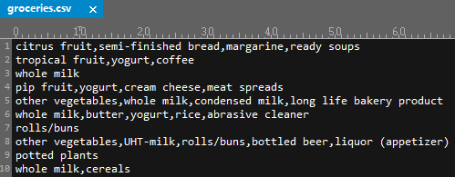
2. as(data.table,'transactions') 函数转化
2.1 若数据存储格式如上图所示也可以通过以下方式读取
trans1 <- as(lapply(fread('./groceries.csv',
                          sep='\t',header = FALSE)$V1,
                    function(x) unlist(strsplit(x,','))),
             'transactions')
> inspect(trans1)[1:3]
     items
[1]  {citrus fruit,
      margarine,
      ready soups,
      semi-finished bread}
[2]  {coffee,
      tropical fruit,
      yogurt}
[3]  {whole milk}
2.2 若数据存储格式如下图所示

trans1 <- as(lapply(interaction(fread(file,sep=',',header = TRUE,
                                     col.names = c('id1',paste('info',1:ncols_good,sep='')))[,!'id1'],sep=','),
                    function(x) unlist(strsplit(as.character(x),','))),
             'transactions')
> inspect(trans1)
    items
[1] {g5,g7,g8}
[2] {g12,g4,g9}
[3] {g11,g6,g7}
[4] {g15,g22,g9}
[5] {g14,g2,g23}
[6] {g13,g24,g8}
[7] {g11,g25,g3}
2.2.1 list转化
> (ls1 <- list(c('w1','w2'),paste('g',1:4,sep=''),c('h1','h2','h8')))
[[1]]
[1] "w1" "w2"

[[2]]
[1] "g1" "g2" "g3" "g4"

[[3]]
[1] "h1" "h2" "h8"

> tr1 <- as(ls1,'transactions')
> inspect(tr1)
    items
[1] {w1,w2}
[2] {g1,g2,g3,g4}
[3] {h1,h2,h8}
3. 读取速度比较
> groceries
transactions in sparse format with
 157360 transactions (rows) and
 169 items (columns)
> system.time(trans1 <- as(lapply(fread('./groceriescopy.csv',sep='\t',header = header)$V1,
                                function(x) unlist(strsplit(x,','))),
                         'transactions'))
 用户  系统  流逝
17.30  0.03 17.34
> system.time(groceries <- read.transactions("groceriescopy.csv", format="basket", sep=",") )
 用户  系统  流逝
41.04  0.13 41.45
数据集及统计汇总信息查看
统计信息查看
> summary(groceries)
transactions as itemMatrix in sparse format with
9835 rows (elements/itemsets/transactions) and
169 columns (items) and a density of 0.02609146

most frequent items:
  whole milk other vegetables       rolls/buns             soda
2513             1903             1809             1715
yogurt          (Other)
1372            34055

element (itemset/transaction) length distribution:
  sizes
1    2    3    4    5    6    7    8    9   10   11   12   13   14   15
2159 1643 1299 1005  855  645  545  438  350  246  182  117   78   77   55
16   17   18   19   20   21   22   23   24   26   27   28   29   32
46   29   14   14    9   11    4    6    1    1    1    1    3    1

Min. 1st Qu.  Median    Mean 3rd Qu.    Max.
1.000   2.000   3.000   4.409   6.000  32.000

includes extended item information - examples:
  labels
1 abrasive cleaner
2 artif. sweetener
3   baby cosmetics
summary的含义:
第一段:总共有9835条交易记录transaction,169个商品item. density=0.026表示在稀疏矩阵中1的百分比
第二段:最频繁出现的商品item,以及其出现的次数. 可以计算出最大支持度.
第三段:每笔交易包含的商品数目,以及其对应的5个分位数和均值的统计信息.如:2159条交易仅包含了1个商品,1643条交易购买了2件商品,一条交易购买了32件商品. 那段统计信息的含义是:第一分位数是2,意味着25%的交易包含不超过2个item. 中位数是3表面50%的交易购买的商品不超过3件. 均值4.4表示所有的交易平均购买4.4件商品
第四段:如果数据集包含除了Transaction Id 和 Item之外的其他的列(如,发生交易的时间,用户ID等等),会显示在这里。这个例子,其实没有新的列,labels就是item的名字
购物车数据的稀疏矩阵形式查看
mx1 <- as(groceries,'matrix')
dim(mx1)
[1] 9835  169
head(mx1[,1:5])
     abrasive cleaner artif. sweetener baby cosmetics baby food  bags
[1,]            FALSE            FALSE          FALSE     FALSE FALSE
[2,]            FALSE            FALSE          FALSE     FALSE FALSE
[3,]            FALSE            FALSE          FALSE     FALSE FALSE
[4,]            FALSE            FALSE          FALSE     FALSE FALSE
[5,]            FALSE            FALSE          FALSE     FALSE FALSE
[6,]             TRUE            FALSE          FALSE     FALSE FALSE
数据集信息进一步查看
> (str(groceries))
Formal class 'transactions' [package "arules"] with 3 slots
  ..@ data       :Formal class 'ngCMatrix' [package "Matrix"] with 5 slots
  .. .. ..@ i       : int [1:43367] 29 88 118 132 33 157 167 166 38 91 ...
  .. .. ..@ p       : int [1:9836] 0 4 7 8 12 16 21 22 27 28 ...
  .. .. ..@ Dim     : int [1:2] 169 9835
  .. .. ..@ Dimnames:List of 2
  .. .. .. ..$ : NULL
  .. .. .. ..$ : NULL
  .. .. ..@ factors : list()
  ..@ itemInfo   :'data.frame': 169 obs. of  1 variable:
  .. ..$ labels: chr [1:169] "abrasive cleaner" "artif. sweetener" "baby cosmetics" "baby food" ...
  ..@ itemsetInfo:'data.frame': 0 obs. of  0 variables
NULL
> (class(groceries))
[1] "transactions"
attr(,"package")
[1] "arules"
> (dim(groceries))
[1] 9835  169
# 每个购物list里包含商品的数量 length in each basket(row)
> basketSize<-size(groceries)
> table(basketSize)
basketSize
   1    2    3    4    5    6    7    8    9   10   11   12   13   14   15   16
2159 1643 1299 1005  855  645  545  438  350  246  182  117   78   77   55   46
  17   18   19   20   21   22   23   24   26   27   28   29   32
  29   14   14    9   11    4    6    1    1    1    1    3    1
# 单个商品的出现频率 Support of each item
> itemFreq <- itemFrequency(groceries)
> (head(itemFreq[order(-itemFreq)]))
      whole milk other vegetables       rolls/buns             soda
       0.2555160        0.1934926        0.1839349        0.1743772
          yogurt    bottled water
       0.1395018        0.1105236
按最小支持度查看
# itemfreq >= 0.1
itemFrequencyPlot(groceries, support= quantile(itemFreq,0.9))

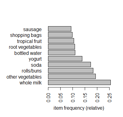
按照支持度的topn查看
# head(itemFreq[order(-itemFreq)],10)
itemFrequencyPlot(groceries, topN=10, horiz=T)
有效数据集筛选
筛选购买两件商品以上的交易
groceries_use <- groceries[basketSize > 1]
dim(groceries)
[1] 9835  169
dim(groceries_use)
[1] 7676  169
查看交易数据
inspect(groceries[1:3])
    items
[1] {citrus fruit,
     margarine,
     ready soups,
     semi-finished bread}
[2] {coffee,
     tropical fruit,
     yogurt}
[3] {whole milk}
关联规则挖掘
groceryrules <- apriori(groceries,
                        parameter = list(support = 0.006,
                                         confidence = 0.25,
                                         minlen = 2))
这里需要说明下parameter:
默认的support=0.1, confidence=0.8, minlen=1, maxlen=10
对于minlen,maxlen这里指规则的LHS+RHS的并集的元素个数
如果minlen=1,意味着 {} => {beer}是合法的规则
我们往往不需要这种规则,所以需要设定minlen=2
解决支持度设定的一种方法是在考虑一个有趣的模式之前,事先想好需要的最小交易数量. 例如
你认为如果某种商品一天被购买2次就可以入法眼, 一个月也就是2x30=60次交易记录,则最小支持度可以计算为 60/9835=0.006即
置信度阙值从0.25开始,意味着将正确规则完全包含在此结果中,其最低准确率也会使25%
规则统计汇总信息
summary(groceryrules)
set of 463 rules

rule length distribution (lhs + rhs):sizes
  2   3   4
150 297  16

   Min. 1st Qu.  Median    Mean 3rd Qu.    Max.
  2.000   2.000   3.000   2.711   3.000   4.000

summary of quality measures:
    support           confidence          lift            count
 Min.   :0.006101   Min.   :0.2500   Min.   :0.9932   Min.   : 60.0
 1st Qu.:0.007117   1st Qu.:0.2971   1st Qu.:1.6229   1st Qu.: 70.0
 Median :0.008744   Median :0.3554   Median :1.9332   Median : 86.0
 Mean   :0.011539   Mean   :0.3786   Mean   :2.0351   Mean   :113.5
 3rd Qu.:0.012303   3rd Qu.:0.4495   3rd Qu.:2.3565   3rd Qu.:121.0
 Max.   :0.074835   Max.   :0.6600   Max.   :3.9565   Max.   :736.0

mining info:
      data ntransactions support confidence
 groceries          9835   0.006       0.25
规则查看
inspect(groceryrules[1:5])
    lhs                rhs                support     confidence lift     count
[1] {potted plants} => {whole milk}       0.006914082 0.4000000  1.565460 68
[2] {pasta}         => {whole milk}       0.006100661 0.4054054  1.586614 60
[3] {herbs}         => {root vegetables}  0.007015760 0.4312500  3.956477 69
[4] {herbs}         => {other vegetables} 0.007727504 0.4750000  2.454874 76
[5] {herbs}         => {whole milk}       0.007727504 0.4750000  1.858983 76
有用规则提取
规则可以划分为3大类
- Actionable 这些rule提供了非常清晰、有用的洞察,可以直接应用在业务上
- Trivial 这些rule显而易见,很清晰但是没啥用。属于common sense,如 {尿布} => {婴儿食品}
- Inexplicable 这些rule是不清晰的,难以解释,需要额外的研究来判定是否是有用的rule
接下来,我们讨论如何发现有用的rule
1. 按照 lift 对规则进行排序
ordered_groceryrules <- sort(groceryrules, by="lift")
inspect(ordered_groceryrules[1:5])
    lhs                   rhs                support
[1] {other vegetables} => {whole milk}       0.07483477
[2] {whole milk}       => {other vegetables} 0.07483477
[3] {rolls/buns}       => {whole milk}       0.05663447
[4] {yogurt}           => {whole milk}       0.05602440
[5] {root vegetables}  => {whole milk}       0.04890696
    confidence lift     count
[1] 0.3867578  1.513634 736
[2] 0.2928770  1.513634 736
[3] 0.3079049  1.205032 557
[4] 0.4016035  1.571735 551
[5] 0.4486940  1.756031 481

groceryrules@quality$lift2 <- floor(groceryrules@quality$lift*100)/100
ordered_groceryrules2 <- sort(groceryrules, by=c("lift2",'support'))
inspect(ordered_groceryrules2[11:16])
    lhs                                             rhs               support
[1] {other vegetables,whole milk,yogurt}         => {root vegetables} 0.007829181
[2] {tropical fruit,whipped/sour cream}          => {yogurt}          0.006202339
[3] {other vegetables,tropical fruit,whole milk} => {yogurt}          0.007625826
[4] {other vegetables,rolls/buns,whole milk}     => {root vegetables} 0.006202339
[5] {other vegetables,tropical fruit}            => {root vegetables} 0.012302999
[6] {frozen vegetables,other vegetables}         => {root vegetables} 0.006100661
    confidence lift     count lift2
[1] 0.3515982  3.225716  77   3.22
[2] 0.4485294  3.215224  61   3.21
[3] 0.4464286  3.200164  75   3.20
[4] 0.3465909  3.179778  61   3.17
[5] 0.3427762  3.144780 121   3.14
[6] 0.3428571  3.145522  60   3.14
2. 规则搜索
yogurtrules <- subset(groceryrules, items %in% c("yogurt"))
inspect(yogurtrules[1:3])
    lhs              rhs      support     confidence lift     count lift2
[1] {cat food}    => {yogurt} 0.006202339 0.2663755  1.909478 61    1.90
[2] {hard cheese} => {yogurt} 0.006405694 0.2614108  1.873889 63    1.87
[3] {butter milk} => {yogurt} 0.008540925 0.3054545  2.189610 84    2.18
items %in% c("A", "B")表示 lhs+rhs的项集并集中,至少有一个item是在c("A", "B") item = A or item = B
如果仅仅想搜索lhs或者rhs,那么用lhs或rhs替换items即可。如:lhs %in% c("yogurt")
%in%是精确匹配
%pin%是部分匹配,也就是说只要item like '%A%' or item like '%B%'
%ain%是完全匹配,也就是说itemset has ’A' and itemset has ‘B'
3. 通过 条件运算符(&, |, !) 添加 support, confidence, lift的过滤条件
fruitrules <- subset(groceryrules, items %pin% c("fruit"))
inspect(sort(yogurtrules[1:3],by=c('lift2','support')))
    lhs                        rhs              support     confidence lift     count lift2
[1] {grapes}                => {tropical fruit} 0.006100661 0.2727273  2.599101  60   2.59
[2] {fruit/vegetable juice} => {soda}           0.018403660 0.2545710  1.459887 181   1.45
[3] {fruit/vegetable juice} => {yogurt}         0.018708693 0.2587904  1.855105 184   1.85

byrules <- subset(groceryrules, items %ain% c("berries"))
inspect(byrules[1:3])
    lhs          rhs                  support     confidence lift     count lift2
[1] {berries} => {whipped/sour cream} 0.009049314 0.2721713  3.796886  89   3.79
[2] {berries} => {yogurt}             0.010574479 0.3180428  2.279848 104   2.27
[3] {berries} => {other vegetables}   0.010269446 0.3088685  1.596280 101   1.59

fruitrules <- subset(groceryrules, items %pin% c("fruit") & lift > 2)
inspect(fruitrules[1:3])
    lhs                 rhs              support     confidence lift     count lift2
[1] {grapes}         => {tropical fruit} 0.006100661 0.2727273  2.599101  60   2.59
[2] {pip fruit}      => {tropical fruit} 0.020437214 0.2701613  2.574648 201   2.57
[3] {tropical fruit} => {yogurt}         0.029283172 0.2790698  2.000475 288   2.00
4. 获取出support,confidence,lift外的其他评价标准
qualityMeasures <- interestMeasure(groceryrules,
                                   measure = c("coverage","fishersExactTest",
                                            "conviction", "chiSquared"),
                                   transactions=groceries_use)
summary(qualityMeasures)
    coverage        fishersExactTest      conviction       chiSquared
 Min.   :0.009964   Min.   :0.0000000   Min.   :0.9977   Min.   :  0.0106
 1st Qu.:0.018709   1st Qu.:0.0000000   1st Qu.:1.1914   1st Qu.: 25.0673
 Median :0.024809   Median :0.0000000   Median :1.2695   Median : 45.6076
 Mean   :0.032608   Mean   :0.0068474   Mean   :1.3245   Mean   : 54.9651
 3rd Qu.:0.035892   3rd Qu.:0.0000026   3rd Qu.:1.4091   3rd Qu.: 75.8146
 Max.   :0.255516   Max.   :0.5881507   Max.   :2.1897   Max.   :350.0989

quality(groceryrules) <- cbind(quality(groceryrules), qualityMeasures)
inspect(head(sort(groceryrules, by = "conviction", decreasing = F)))
    lhs                      rhs          support     confidence lift      count lift2
[1] {bottled beer}        => {whole milk} 0.020437214 0.2537879  0.9932367 201   0.99
[2] {bottled water,soda}  => {whole milk} 0.007524148 0.2596491  1.0161755  74   1.01
[3] {beverages}           => {whole milk} 0.006812405 0.2617188  1.0242753  67   1.02
[4] {specialty chocolate} => {whole milk} 0.008032537 0.2642140  1.0340410  79   1.03
[5] {candy}               => {whole milk} 0.008235892 0.2755102  1.0782502  81   1.07
[6] {sausage,soda}        => {whole milk} 0.006710727 0.2761506  1.0807566  66   1.08
    coverage   fishersExactTest conviction chiSquared
[1] 0.08052872 0.5881507        0.9976841  0.01055431
[2] 0.02897814 0.5085760        1.0055826  0.02057106
[3] 0.02602949 0.4684027        1.0084016  0.04149042
[4] 0.03040163 0.4363886        1.0118214  0.09572128
[5] 0.02989324 0.2669417        1.0275976  0.49707571
[6] 0.02430097 0.3180790        1.0285068  0.42791924
第三个参数transactions:一般情况下都是原来那个数据集,但也有可能是其它数据集,用于检验这些rules在其他数据集上的效果。所以,这也是评估rules的一种方法:在其它数据集上计算这些规则的quality measure用以评估效果。
fishersExactTest 的p值大部分都是 >= 0.05, 这就说明这些规则反应出了真实的用户的行为模式。
coverage从0.01 ~ 0.30,相当于覆盖到了多少范围的用户。
ChiSquared: 考察该规则的LHS和RHS是否独立?即LHS与RHS的列联表的ChiSquare Test。p<0.05表示独立,否则表示不独立。
限制挖掘的item
可以控制规则的左手边或者右手边出现的item,即appearance。但尽量要放低支持度和置信度
> berriesInLHS <- apriori(groceries,
                        parameter = list( support = 0.003,
                                          confidence = 0.1,
                                          minlen=2),
                        appearance = list(lhs = c("berries"),
                                          default="rhs"))
> summary(berriesInLHS)
set of 18 rules

rule length distribution (lhs + rhs):sizes
 2
18

   Min. 1st Qu.  Median    Mean 3rd Qu.    Max.
      2       2       2       2       2       2

summary of quality measures:
    support           confidence          lift           count
 Min.   :0.003660   Min.   :0.1101   Min.   :1.081   Min.   : 36.00
 1st Qu.:0.004118   1st Qu.:0.1239   1st Qu.:1.457   1st Qu.: 40.50
 Median :0.005186   Median :0.1560   Median :1.596   Median : 51.00
 Mean   :0.006231   Mean   :0.1874   Mean   :1.791   Mean   : 61.28
 3rd Qu.:0.007168   3rd Qu.:0.2156   3rd Qu.:1.950   3rd Qu.: 70.50
 Max.   :0.011795   Max.   :0.3547   Max.   :3.797   Max.   :116.00

mining info:
      data ntransactions support confidence
 groceries          9835   0.003        0.1

> inspect(berriesInLHS[1:5])
    lhs          rhs                     support     confidence lift
[1] {berries} => {beef}                  0.004473818 0.1345566  2.564659
[2] {berries} => {butter}                0.003762074 0.1131498  2.041888
[3] {berries} => {domestic eggs}         0.003863752 0.1162080  1.831579
[4] {berries} => {fruit/vegetable juice} 0.003660397 0.1100917  1.522858
[5] {berries} => {whipped/sour cream}    0.009049314 0.2721713  3.796886

# 既然lhs都是"berries",那么只查看rhs的itemset即可
> inspect(rhs(berriesInLHS[1:5]))
    items
[1] {beef}
[2] {butter}
[3] {domestic eggs}
[4] {fruit/vegetable juice}
[5] {whipped/sour cream}

# 使用subset进行进一步过滤. 如,不希望看到rhs包含"root vegetables" 或 "whole milk"
> berrySub <- subset(berriesInLHS, subset = !(rhs %in% c("root vegetables", "whole milk")))
> inspect(sort(berrySub, by="confidence")[1:5])
    lhs          rhs                  support     confidence lift     count
[1] {berries} => {yogurt}             0.013548723 0.3280757  1.890622  104
[2] {berries} => {other vegetables}   0.013157895 0.3186120  1.328444  101
[3] {berries} => {whipped/sour cream} 0.011594581 0.2807571  3.173920   89
[4] {}        => {other vegetables}   0.239838458 0.2398385  1.000000 1841
[5] {berries} => {soda}               0.009379885 0.2271293  1.118310   72
> inspect(rhs(sort(berrySub, by="confidence")[1:5]))
    items
[1] {yogurt}
[2] {other vegetables}
[3] {whipped/sour cream}
[4] {other vegetables}
[5] {soda}
保存挖掘的结果
有两种使用场景。
第一,保存到文件。可以与外部程序进行交换。
> write(groceryrules, file="./groceryrules.csv", sep=",", quote=TRUE, row.names=FALSE)
第二,转换为data frame,然后再进行进一步的处理。处理完的结果可以保存到外部文件或者数据库。
> groceryrules_df <- as(groceryrules, "data.frame")
> str(groceryrules_df)
图形展示
1. Scatter Plot
> library(arulesViz)
> library(RColorBrewer)
> plot(groceryrules,
     control=list(jitter=2,col=rev(brewer.pal(9, "Greens")[4:9])),
     shading = 'lift')
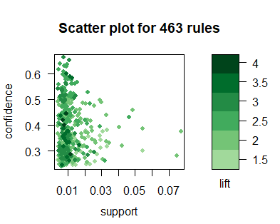
shading = "lift": 表示在散点图上颜色深浅的度量是lift。当然也可以设置为support 或者Confidence
jitter=2:增加抖动值
col: 调色板,默认是100个颜色的灰色调色板
brewer.pal(n, name): 创建调色板:n表示该调色板内总共有多少种颜色;name表示调色板的名字(参考help)
这里使用Green这块调色板,引入9中颜色
这幅散点图表示了规则的分布图:大部分规则的support在0.1以内,Confidence在0-0.8内。每个点的颜色深浅代表了lift的值
2. Grouped Matrix
plot(groceryrules,method='grouped',
     control = list(col=rev(brewer.pal(9, "Greens")[4:9])))

3. Graph
top.vegie.rules <- sort(groceryrules,
                        by=c('support','lift'))[1:10]
plot(top.vegie.rules, measure="support",
     method="graph",
     shading = "lift")

购物篮分析的结果应用
- 通过商品合并购买来揣测我的用户。通过商品一级品类的购物篮分析,发现用户经常购买的是水果和乳品,这两款品种十分契合下午茶场景,说明我们的用户群体中,是办公室白领、比较喜欢下午茶的人群比例有多少。其次是果蔬+乳品,这两款品种十分契合居家生活场景,说明在我们的用户群体中,做饭居家的用户比例有多少。这只是给公司各级别的同事一个基础的数据概念。
- 有了这些数据佐证,我们一方面可以告诉商品在这几类品种上,不断扩品和扩类,另一方面可以指导运营,在合适的时间(下午茶时间和下班买菜时间)进行合适的品类秒杀和促销。
- 优惠券策略。如果要发放优惠券撬动销售额,那么发放什么品类优惠券合适?如果要进行促销,那么促销品中加入哪款商品能促进该促销品的销售?
- 如果运营要制定下午茶活动,或者是菜市场活动,选那些品比较合适?为什么要制定这么场景类的活动?
- 根据起飞价,来制定爆款品定价,坚决不让爆款品组合刚好够起飞价
References:
- R语言 | 关联规则
- 机器学习与R语言-基于关联规则的购物篮分析.P172
- 用R语言进行购物篮分析
- R语言数据挖掘-2.2购物篮分析
- 购物篮关联分析-R挖掘Apriori算法
- R语言学习之关联规则算法