参数展开
在Octave中,若我们需要使用fminuc函数来计算使得代价函数最小化的权重矩阵,我们需要将参数矩阵展开为向量,利用相关算法计算时再将其转换回矩阵。
例如:
- 创建Θ(1),Θ(2),Θ(3)矩阵
octave:1> Theta1 = ones(10, 11);
octave:2> Theta2 = ones(10, 11);
octave:3> Theta3 = ones(1, 11);
octave:4> whos
Variables in the current scope:

   Attr Name        Size                     Bytes  Class
   ==== ====        ====                     =====  =====
        Theta1     10x11                       880  double
        Theta2     10x11                       880  double
        Theta3      1x11                        24  double

Total is 231 elements using 1784 bytes
- 展开参数矩阵
octave:5> thetaVec = [Theta1(:); Theta2(:); Theta3(:)];
octave:6> whos
Variables in the current scope:

   Attr Name          Size                     Bytes  Class
   ==== ====          ====                     =====  =====
        Theta1       10x11                       880  double
        Theta2       10x11                       880  double
        Theta3        1x11                        24  double
        thetaVec    231x1                       1848  double

Total is 462 elements using 3632 bytes
- 计算时,转回Θ(1),Θ(2),Θ(3)矩阵
octave:7> Theta1_r = reshape(thetaVec(1:110), 10, 11);
octave:8> Theta2_r = reshape(thetaVec(111:220), 10, 11);
octave:9> Theta3_r = reshape(thetaVec(221:231), 1, 11);
octave:10> whos
Variables in the current scope:

   Attr Name          Size                     Bytes  Class
   ==== ====          ====                     =====  =====
        Theta1       10x11                       880  double
        Theta1_r     10x11                       880  double
        Theta2       10x11                       880  double
        Theta2_r     10x11                       880  double
        Theta3        1x11                        24  double
        Theta3_r      1x11                        88  double
        thetaVec    231x1                       1848  double

Total is 693 elements using 5480 bytes
- 使用向前或向后传播算法,计算代价函数和下降梯度
补充笔记
Implementation Note: Unrolling Parameters
With neural networks, we are working with sets of matrices:
In order to use optimizing functions such as "fminunc()", we will want to "unroll" all the elements and put them into one long vector:
thetaVector = [ Theta1(:); Theta2(:); Theta3(:); ]
deltaVector = [ D1(:); D2(:); D3(:) ]
If the dimensions of Theta1 is 10x11, Theta2 is 10x11 and Theta3 is 1x11, then we can get back our original matrices from the "unrolled" versions as follows:
Theta1 = reshape(thetaVector(1:110),10,11)
Theta2 = reshape(thetaVector(111:220),10,11)
Theta3 = reshape(thetaVector(221:231),1,11)
To summarize:
梯度检验
当我们对处理一些复杂的模型(如神经网络模型)使用梯度下降算法时,可能存在一些不易发现的错误,虽然代价函数在不断减小,但其最终结果不一定为最优解。
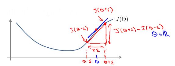
为了避免这样的问题,我们引入梯度的数值检验方法。在介绍梯度下降算法时,我们知道对代价函数J(θ)求θj的偏导数,实质上是θj该点处的切线的斜率。因此,我们可以使用如下方法对该点处的切线的斜率进行近似操作:
其中ε足够小,通常选取10-4。通过该近似值与使用向后传播算法得出的下降梯度值相比较。
对于向量θ而言,其计算方法为:
在Octave中,其代码基本为:
补充笔记
Gradient Checking
Gradient checking will assure that our backpropagation works as intended. We can approximate the derivative of our cost function with:
With multiple theta matrices, we can approximate the derivative with respect to Θj as follows:
A small value for ϵ (epsilon) such as ϵ=10−4, guarantees that the math works out properly. If the value for ϵ is too small, we can end up with numerical problems.
Hence, we are only adding or subtracting epsilon to the Θj matrix. In octave we can do it as follows:
epsilon = 1e-4;
for i = 1:n,
  thetaPlus = theta;
  thetaPlus(i) += epsilon;
  thetaMinus = theta;
  thetaMinus(i) -= epsilon;
  gradApprox(i) = (J(thetaPlus) - J(thetaMinus))/(2*epsilon)
end;
We previously saw how to calculate the deltaVector. So once we compute our gradApprox vector, we can check that gradApprox ≈ deltaVector.
Once you have verified once that your backpropagation algorithm is correct, you don't need to compute gradApprox again. The code to compute gradApprox can be very slow.
随机初始化
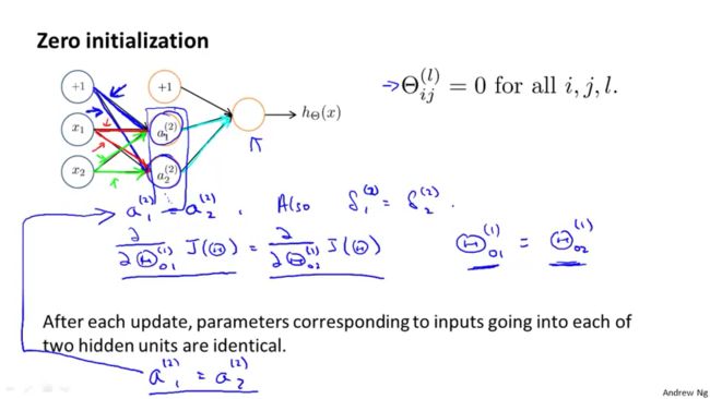
在线性回归和逻辑回归中,我们在使用梯度下降算法或其他高级算法时,我们通常将参数θ初始化为0。但在神经网络模型中,如若我们将参数(权重)θ都初始化为0,那么我们不能得到一个正确的结果。
即使我们将权重θ初始化一个非0的数值,其结果仍旧是错误的。以上图为例,隐藏层的所有激活单元其数值仍然相同。
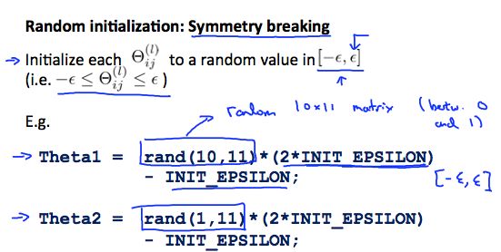
因此,我们需要对权重θ进行随机初始化。
其中,上图中ε与梯度下降检验中的ε无关。
补充笔记
Random Initialization
Initializing all theta weights to zero does not work with neural networks. When we backpropagate, all nodes will update to the same value repeatedly. Instead we can randomly initialize our weights for our Θ matrices using the following method:
Hence, we initialize each Θij(l) to a random value between[−ϵ,ϵ]. Using the above formula guarantees that we get the desired bound. The same procedure applies to all the Θ's. Below is some working code you could use to experiment.
If the dimensions of Theta1 is 10x11, Theta2 is 10x11 and Theta3 is 1x11.

Theta1 = rand(10,11) * (2 * INIT_EPSILON) - INIT_EPSILON;
Theta2 = rand(10,11) * (2 * INIT_EPSILON) - INIT_EPSILON;
Theta3 = rand(1,11) * (2 * INIT_EPSILON) - INIT_EPSILON;
rand(x,y) is just a function in octave that will initialize a matrix of random real numbers between 0 and 1.
(Note: the epsilon used above is unrelated to the epsilon from Gradient Checking)
神经网络算法总结
首先,我们需要选择神经网络模型的结构,即决定神经网络的层数及每一层的激活单元数。
- 输入层(即第一层)的激活单元数为训练集的特征变量数
- 输出层(即最后一层)的激活单元数为分类数
- 隐藏层数大于1时,应确保隐藏层的每层的激活单元数相同,通常情况下隐藏层的激活单元越多越好
神经网络模型训练步骤:
- 随机初始化权重矩阵Θ;
- 利用正向传播算法计算假设函数hΘ(x);
- 编写计算代价函数J(Θ)的代码;
- 利用方向传播算法计算代价函数J(Θ)的偏导数,从而计算出下降梯度;
- 利用梯度检验法(即数值检验法)对下降梯度进行检验;
- 利用优化算法(如梯度下降算法或其他高级优化算法)计算出使得代价函数J(Θ)最小化的权重矩阵Θ。
注:神经网络模型中的代价函数J(Θ)为非凸(国内非凹)函数。因此,所求得的权重矩阵Θ为代价函数J(Θ)的局部最优解。
补充笔记
Putting it Together
First, pick a network architecture; choose the layout of your neural network, including how many hidden units in each layer and how many layers in total you want to have.
- Number of input units = dimension of features x(i)
- Number of output units = number of classes
- Number of hidden units per layer = usually more the better (must balance with cost of computation as it increases with more hidden units)
- Defaults: 1 hidden layer. If you have more than 1 hidden layer, then it is recommended that you have the same number of units in every hidden layer.
Training a Neural Network
- Randomly initialize the weights
- Implement forward propagation to get hΘ(x(i)) for any x(i)
- Implement the cost function
- Implement backpropagation to compute partial derivatives
- Use gradient checking to confirm that your backpropagation works. Then disable gradient checking.
- Use gradient descent or a built-in optimization function to minimize the cost function with the weights in theta.
When we perform forward and back propagation, we loop on every training example:
for i = 1:m,
   Perform forward propagation and backpropagation using example (x(i),y(i))
   (Get activations a(l) and delta terms d(l) for l = 2,...,L
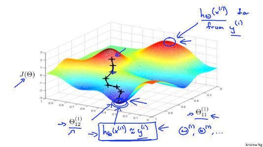
The following image gives us an intuition of what is happening as we are implementing our neural network:
Ideally, you want hΘ(x(i)) ≈ y(i). This will minimize our cost function. However, keep in mind that J(Θ) is not convex and thus we can end up in a local minimum instead.


