Discovery the motivation of behavior from electricity consumption signal
Key Points
This chapter briefly elaborates how to analyze the motivation of people's operation on a system from the system electricity consumption signal and other data.
Objective: understand how, and why occupants interact with the system.
System: ventilation system in passive houses with adjustable flow rate option.
Raw data: electricity consumption signal; environment sensor records (temperature, humidity, CO2 etc.); 3-min interval * 2 years (2013-2015): 325946 rows × 25 features.
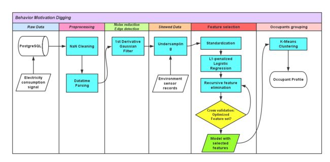
Below Figure 1 shows the overall pipeline I designed.
flowchart
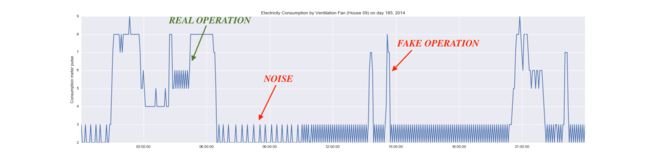
(1) After essential preprocessing and cleaning (NaNs are backfilled), start with a system electricity consumption signal like Figure 2 below. A sudden change in the signal could imply the occupants' interaction with the system (e.g. once the occupant turn the flow rate into a higher option there should be a steep increasing edge on the electricity consumption signal). First thing to do is filtering out the noise (caused by wind etc. or system itself) and "fake operation" (status change with too-short duration).
Figure 2 Demo of Electricity Consumption Signal
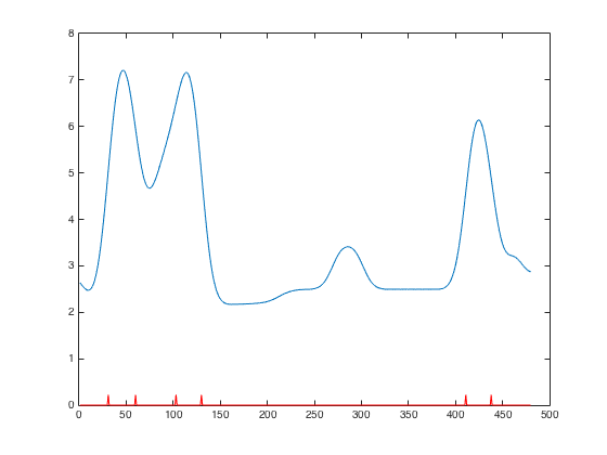
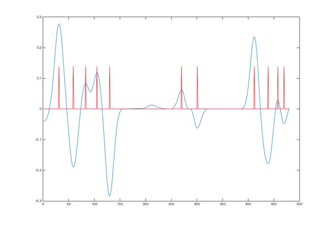
(2) Through a finely-tuned 1st derivative Gaussian filter, the noise and "fake operation" could be filtered out and the valid operations would be marked out, like shown in Figure 3 below.
Noise reduced signal
1st Derivative filtered signal
Operation Marked
(3) Then the marked data set would undergo an undersampling process since the dataset is now skewed (The no. of records marked with 'no operation' is far more than ones with operation, either increase or decrease). The undersampling process ensures the data set has balanced scales with each class, for the effectiveness of following classification algorithm.
(4) After undersampling, the training set would be normalized and then fed into a L1-penalized logistic regression classifier. Since linear model penalized with L1 norm has sparse solutions i.e. many of its estimated coefficients would be zero, it could be used for feature selection purpose. Figure 4 below shows an example of the coefficients output in a certain experiment.
Coefficient output of logistic regression model
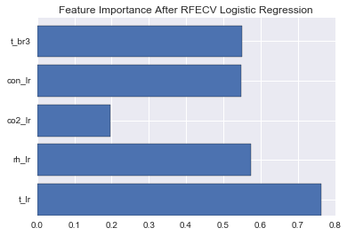
Then the logistic regression runs repeatedly to make a recursive feature elimination (first, the estimator is trained on the initial set of features and weights are assigned to each one of them. Then, features whose absolute weights are the smallest are pruned from the current set features). At last, the most informative feature combination (judged by cross-validation accuracy) in this case could be determined, like below Figure 5 shows: these features implies this occupant's motivation for his/her behavior.
Best feature combination after recursive feature elimination
(5) Repeat the process above for different occupants. The results imply there are different kinds of people since their "best feature combination" vary a lot: e.g. some of them are with strong "time pattern" while others may be more sensitive to indoor environment, like temperature etc. A K-Means clustering could help us demonstrate this by grouping the occupants into different user profiles.
Grouping: different user profiles found
From here below is technical log regarding relevant theory and code to realize the whole process.
There is a ventilation system (with heat recovery) in one passive house, of which the ventilation flow rate is controlled by a fan system, and adjustable by occupants. There are 3 available options (let's say, low, medium, high rate respectively)for the fan flow rate setting.
The electricity consumption of the fan system is recorded by a smart meter in terms of pulse. Obviously, occupants' flow rate setting could put significant influence on the electricity consumption and we could calibrate when and how people adjust their ventilation system based on the electricity consumption.
However, on the one hand, with the influence of back pressure, wind speed etc. the record is not something like a clear 3-stage square wave, instead it is quite noisy. On the other hand, we got many different houses (with similar structure but with different scales of records) within our research. They made it is not really practical to calibrate the ventilation setting position by fixed intervals (like pulse < 3 == position 1; 3 < pulse < 5 == position 2 etc.). We need a new algorithmic method to do this job.
This is a tiny piece of the elec. consumption record (day 185 in year 2014, house #9):
Methodology
Describe what we want to do in a few words: smooth the noise and detect the edge automatically, without any reset like boundary interval needed. This is actually a classic problem in signal processing or computer vision field. For this 1D signal the simplest solution maybe Gaussian derivative filter, for similar problems in 2D matrix (images) the canny edge detector could be effective. The figure may give you a vivid impression of what we are going to do:
Basic idea
Tune a Gaussian derivative filter to properly smooth the noise and take 1st derivative, then set an appropriate threshold to detect the edge.
Terms
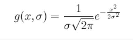
Gaussian filter
For noise smoothing or "image blur". In layman's words, replace each point by the weighted average of its neighbors, the weights come from Gaussian distribution, then normalize the results.
Gaussian
(if you are dealing with 2d matrix (images), use 2-D Gaussian instead.)
Effect:
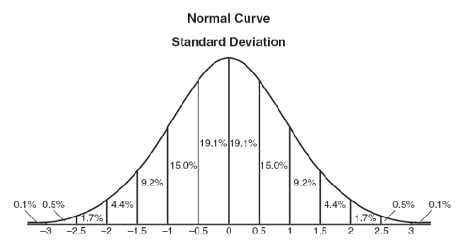
Gaussian derivative filter
For noise smoothing and edge detection. In layman's words, replace each point by the weighted average of its neighbors, the weights come from the 1st derivative of Gaussian distribution, then normalize the results.
Effect:
Advantages of Gaussian Kernel compared to other low-pass filter:
Being possible to derive from a small set of scale-space axioms.
Does not introduce new spurious structures at coarse scales that do not correspond to simplifications of corresponding structures at finer scales.
Scale Space
Representing an signal/image as a one-parameter family of smoothed signals/images, parametrized by the size of the smoothing kernel used for suppressing fine-scale structures. Specially for Gaussian kernels: t = sigma^2.
Results
Finished a demo of auto edge detection in our elec. consumption record, which contains a tuned Gaussian derivative filter, edge position detected, and scale space plot.
Original
Gaussian filter smoothed (sigma = 8)
1st derivative Gaussian filtered (sigma = 8)
Edge position detected (threshold = 0.07 * global min/max)
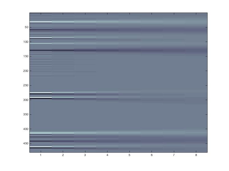
Scale Space (sigma = range (1,9))
Finer Tuning
In practice, it is usually needed to use different tailored tune strategies for the parameters to meet the specific requirements aroused by researchers. E.g. in a case the experts from built environment would like to filter out short-lived status (even they maybe quite steep in terms of pulse number). The strategies is carefully increase sigma (by which you are flattening the Gaussian curve, so the weights of center would be less significant so that the short peaks could be better wiped out by its flat neighbors) and also, properly increase the threshold would help (by which it would be more difficult for the derivatives of smoothed short peaks to pass the threshold and be recognized as one effective operation). Once the sigma and threshold reached an optimized combination, the results would be something like below for this case:
Edge position detected (Sigma = 10, threshold = 0.35 * global min/max)
In a larger scale, see how does our finely-tuned lazy filter work to filter the fake operations out! (Sigma = 20, threshold = 0.5 * global min/max)
Reference
Scale Space wiki
Gaussian Blur Algorithm
OpenCV Canny Edge Detector
UNC Edge Detector 1D
scikit-image Canny edge detector
Technical Details: Feature selection
Before feature selection I made an undersampling to the data set to ensure every class shares a balanced weight in the whole dataset (before which the ratio is something like 150,000 no operation, 400 increase, 400 decrease).
The feature selection process is carried out in Python with scikit-learn. First each feature in the data set need to be standardized since the objective function of the l1 regularized linear model we use in this case assumes that all features are centered on zero and have variance in the same order. If a feature has a significantly lager scale or variance compared to others, it might dominate the objective function and make the estimator unable to learn from other features correctly as expected. In this case I used sklearn.preprocessing.scale() to standardize each feature to zero mean and unit variance.
Then the standardized data set was fed into a recursive feature elimination with cross-validation (REFCV) loop with a L1-penalized logistic regression kernel since linear models penalized with the L1 norm have sparse solutions: many of their estimated coefficients are zero, which could be used for feature selection purpose.
Below is the main part of the coding script for this session (ipynb format).
Feature selection after Gaussian filter
import matplotlib.pyplot as plt
%matplotlib inline
import numpy as np
import pandas as pd
import seaborn as sns
import math
undersampled_up = pd.concat([up_sample,noop_sample])
undersampled_up.head()
#generate month/hour attribute from datetime string
undersampled_up.dt = pd.to_datetime(undersampled_up.dt)
t = pd.DatetimeIndex(undersampled_up.dt)
hr = t.hour
undersampled_up['HourOfDay'] = hr
month = t.month
undersampled_up['Month'] = month
year = t.year
undersampled_up['Year'] = year
undersampled_up.head()
for col in undersampled_up:
    print col
def remap(x):
    if x == 't':
        x = 0
    else:
        x = 1
    return x

for col in ['wc_lr', 'wc_kitchen', 'wc_br3', 'wc_br2', 'wc_attic']:
    w = undersampled_up[col].apply(remap)
    undersampled_up[col] = w
undersampled_up.head()
openwin = undersampled_up.wc_attic + undersampled_up.wc_br2 + undersampled_up.wc_br3 + undersampled_up.wc_kitchen + undersampled_up.wc_lr
undersampled_up['openwin'] = openwin;
undersampled_up = undersampled_up.drop(['wc_lr', 'wc_kitchen', 'wc_br3', 'wc_br2', 'wc_attic','Year','dt','pulse_channel_ventilation_unit'],axis = 1)
undersampled_up.head()
for col in undersampled_up:
    print col
Logistic Regression
from sklearn.linear_model import LogisticRegression
from sklearn.feature_selection import SelectFromModel
#shuffle the order
undersampled_up = undersampled_up.reindex(np.random.permutation(undersampled_up.index))
undersampled_up.head()
y = undersampled_up.pop('op')
# Columnwise Normalizaion
from sklearn import preprocessing
X_scaled = pd.DataFrame()
for col in undersampled_up:
    X_scaled[col] = preprocessing.scale(undersampled_up[col])
X_scaled.head()
from sklearn import cross_validation
lg = LogisticRegression(penalty='l1',C = 0.1)
scores = cross_validation.cross_val_score(lg, X_scaled, y, cv=10)
#The mean score and the 95% confidence interval of the score estimate
print("Accuracy: %0.2f (+/- %0.2f)" % (scores.mean(), scores.std() * 2))
web.xml报错
The content of element type "web-app" must match "(icon?,display-
name?,description?,distributable?,context-param*,filter*,filter-mapping*,listener*,servlet*,s
JUnit4:Test文档中的解释:
The Test annotation supports two optional parameters.
The first, expected, declares that a test method should throw an exception.
If it doesn't throw an exception or if it
借鉴网上的思路,用java实现:
public class NoIfWhile {
/**
* @param args
*
* find x=1+2+3+....n
*/
public static void main(String[] args) {
int n=10;
int re=find(n);
System.o
在Linux中执行.sh脚本,异常/bin/sh^M: bad interpreter: No such file or directory。
分析:这是不同系统编码格式引起的:在windows系统中编辑的.sh文件可能有不可见字符,所以在Linux系统下执行会报以上异常信息。
解决:
1)在windows下转换:
利用一些编辑器如UltraEdit或EditPlus等工具
Binary search tree works well for a wide variety of applications, but they have poor worst-case performance. Now we introduce a type of binary search tree where costs are guaranteed to be loga