Data Processing Architecture of GraphLab Create

Data Processing Architecture of GraphLab Create

Introduction/Design Philosophy

As the person responsible for architecting the backend data processing architecture ofGraphLab Create, I try to figure out what can we provide to streamline a data scientist’s process“From Inspiration to Production”. And there is much to do. As it turns out supporting all of data science is a non-trivial endeavor. Who knew? :-)

The way I attack complicated problems like “how do we build a system to do X”, is to not actually attack the problem directly. But instead address the indirect question “what is the abstraction we need that will allow us to build a system that does X?” By addressing the “abstraction” question, we can end up with an architecture that is far more generalizable, and way more useful.

For instance: Instead of “how do we solve PageRank quickly?”, ask the question “what is the abstraction that will allow us to solve PageRank quickly?”. The gap between the two questions is the difference between a dedicated implementation of a PageRank solver, and PowerGraph: which solves far more problems.

I'd rather write programs to write programs than write programs

-- Dick Sites (DEC), quoted by Jon Bentley inMore Programming Pearls (1988)

We are not just writing ML algorithms. Instead, we are building abstractions that can help with scalable ML algorithms.

We are not just implementing distributed ML. Instead, we are building distributed abstractions that can help with distributed ML.

It means that it we might take a little longer to get there; but when we do, it will be game changing.

SFrame

One of the core foundational data structures in GraphLab Create is the SFrame. What is the SFrame? An SFrame is in brief, a columnar, table data structure: similar in nature, and very much inspired by the Pandas DataFrame, or the R DataFrame. However, the key difference is that the SFrame is architected around the needs of data science.

These were the design requirements:

1: Efficient Columnar Access And Manipulation

In data science, the ability to access, manipulate, individual columns are crucial.

For instance:

I want to be able to compute individual columnar statistics.

I want to identify and truncate outlier values within a single feature.

I want to run regressions over subsets of columns to identify unnecessary columns.

I want to normalize a column.

I want to generate new feature columns.

Efficient access to individual columns is necessary. (It is no coincidence that Pandas and R DataFrames are columnar in design).

2: SQL-like Query Operations

One tends to have many data sources which you have to explore and combine in different ways. Classical SQL-like query operations such asjoins, andgroup by aggregatesare very useful for data understanding. However, we do not need transactional capability, nor do we need fine-grained table mutations. In other words, we do not need a transactional database, but batch operations (like Pig, Hive, Spark) are sufficient.

3: Strong and Weak Schemas

While strong schemas are desirable for many ML algorithms (for instance it is useful to guarantee a priori that the “rating” column I am trying to predict are all integers), initial real world data processing includes a lot of weak, or flexible schema types (JSON for instance). We need to be able to support both strong and weak schemas.

This design permits highly flexible feature engineering. For instance, a simple spam filtering algorithm could simply taking documents as input, generating a bag of words from each document and performing regression. This requires conversion of string input to a dictionary, and the ability to perform regression on arbitrary dictionary values.

While strong recursive schemas (such as that used by Parquet) is architecturally beautiful (and definitely the right design for the task they are solving), weak schemas provide a large degree of flexibility especially when exploring an unknown datasource. Through the development of GraphLab Create, we have worked with many companies, and the myriad of interesting formats we have encountered makes this extremely valuable. We may load the data first into a weak-schema type representation: then perform feature engineering to extract individual strong schema features.

4: Memory Should Not be a Limiting Factor

I want to be able to explore and manipulate reasonably large quantities of data entirely from my work laptop / desktop without requiring a cluster. If the data does not fit in memory, of course data subsampling can be done, but one basic rule of data science is “the more data the better”. I should not be limited by my memory capacity.

Also, to support data science in production, we need scalability and stability. The same job which runs successfully on 1% of the data should similarly complete on 100% of the data. Jobs should not fail due to resource limits.  When I worked with Hadoop previously, the most annoying issue I have was trying to figure out the right value for the JVM heap size, and this thus became a major pet peeve.

5: Very Large Number Of Columns

An earlier design of the SFrame only supported relatively few columns (<=100). The thought process then was “If you have data with >100 columns, it is probably machine generated, in which a dense/sparse-vector representation in a single column is better”.

But as it turns out people do have data with thousands of columns (we have seen a 100K column case). While the above statement is probably still true, in auser’s firstphilosophy, wemustbe able to handle and process the user’s data. Thus, the ability to handle a very large number of columns is one of the design objectives.

SFrame Design

The SFrame design must take into consideration all the above requirements but there are other less obvious requirements which impact the design (for instance, supporting thousands of columns, random row access, etc). The current architecture is called SFrame v2 and is what I am going to describe here.

Immutability

The first design decision for the SFrame internal representation, is “immutability”. In other words, the SFrame file format can only be written to once, and cannot be updated/modified without rewriting the entire file. There are a few reasons for this decision.

HDFS does not support random writes.

We don’t have to worry about transactions, data sharing, multiple writers, corruption, etc.

Immutable write-once file formats are easier to design and implement, and allows us to focus simply on bulk throughput performance.

However, most importantly, an immutable representation allows lazy evaluation + query optimization to be built much more easily since we are guaranteed that the input which the query depends on is not changing.

However, while the file format is immutable, this does not mean adding new columns to an existing SFrame requires a full rewrite (supporting this case efficiently is indeed one of the design objectives). To see how this is implemented, we must look at the deeper object design.

Object Design

There are 3 key objects involved in the internal SFrame design:

SArrayGroup: The SArrayGroup implements the physical representation of an immutable collection of columns on disk.

SArray: The SArray provides access to a single immutable typed column of data. The SArray is simply a reference to a column inside anSArrayGroup.

SFrame: The SFrame provides access to a table (a collection of columns of all the same length) where each column is just anSArrayobjects.

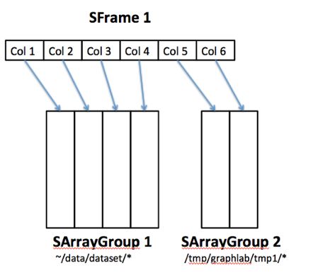
Here is an example of how an SFrame may be structured. This is an SFrame of 6 columns where the first 4 come from one SArrayGroup and 2 come from another SArrayGroup.

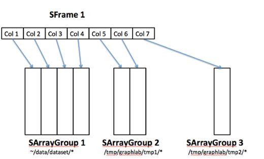
The logical nature of the SFrame thus permits new columns to be added easily without data rewrites, by simply creating new SArrayGroups. here we add a new column to the SFrame (col 7) pointing to new SArrayGroup.

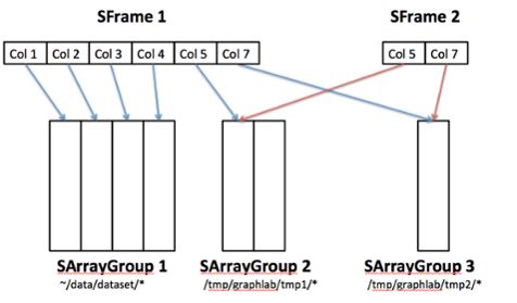
And similarly columns of the SFrames can also be deleted easily without any data rewrites. Here, the deletion of column 6 is performed by simply removing the reference to it.

Column subselection can also be done easily by simply creating a new SFrame pointing to a subset of the columns in the original SFrame. This is safe since SArrayGroups are immutable. “Modification” of columns is basically performed by creation of new SArrayGroups and updating the SFrame/SArray references.

The SFrame and the SArray are hence very simple data structures: they just contain references to SArrayGroups. The key to obtaining good performance is in the implementation of the SArrayGroup.

SArrayGroup

The SArrayGroup implements the actual on disk encoding of a collection of columns of the same length. The ArrayGroup is represented as a collection of files (you can see this by saving an SFrame and looking in the saved directory):

-[prefix].sidx: The index file which contains basic metadata (the column lengths, datatypes, etc)

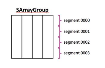
-[prefix].0000, [prefix].0001 … [prefix].NNNN: The segment files. Each segment represents a contiguous subset of rows in the ArrayGroup. For instance, if the ArrayGroup has 100 rows, and there are 5 segments,  [prefix].0000 may contain the first 20 rows, [prefix].0001 may contain the next 20 rows, and so on, until [prefix].0004 will contain the last 20 rows. The division of number of rows in each segment need not be uniform.

The use of segmentation is to simply provide parallel write capability, since each segment file can be written independently by different threads/processes/machines. The ArrayGroup however, provides random read capability so even if the ArrayGroup has only one large segment, it can be read in parallel by an arbitrary number of threads.

SArrayGroup Segment

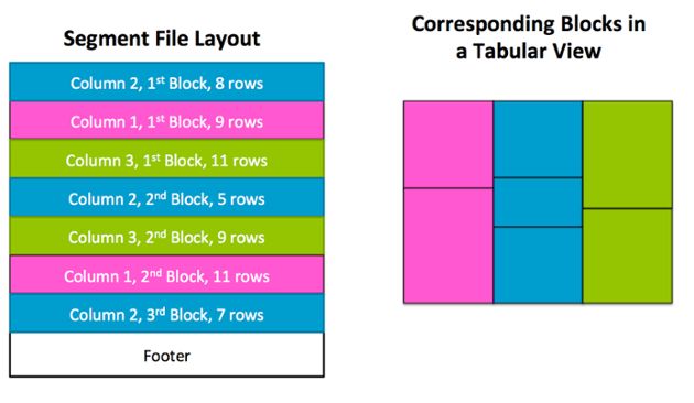
The segment internally is simply an collection of blocks, where each block is a contiguous range of rows within a single column. A file footer contains a descriptor of the file offsets of each block, the column the block belongs to, and the number of rows in each block.

Observe that unlike Parquet or RCFile which horizontally partitions the table into row groups, in the SArrayGroup the blocks do not have to be row-aligned, but instead allowing each column to have a completely different block layout. Columns which are easier to compress to be encoded with much fewer blocks and thus allows us to provide very high throughput on single column scans. The tradeoff however, is that random row access is much more costly since blocks are not aligned and have to be decoded and consumed at different rates. However, since efficient random row access is not a design objective, this tradeoff was considered desirable. (In any case, since SFrames can span multiple ArrayGroups, which may not be block aligned with each other, there is not reason to require alignment within one ArrayGroup).

The blocking strategy is to try to pack as many values into a block as possible, so that thecompressedsize of the block is approximately 64KB (This is a soft limit). We estimate the number of values that can be packed in 64KB compressed by tracking the compression ratios of previous blocks and assuming that future values can be compressed at the same ratio.

Block Encoding

The SFrame currently supports the following datatypes for each column:

integer

double

string

array of doubles

list of arbitrary types

dictionary of arbitrary types

I will only discuss the encoding strategies for 3 of the basic types here. Integer, Double and String.

Integers

Blocks of integers are encoded with whichever of the following provide the smallest representation.

Frame Of Reference encoding (differences to a minimum value)

Delta encoding (incremental differences).

Delta encoding with negative deltas (incremental differences, but with potentially negative deltas)

The encoder implementation is relatively fast, encoding about 300M integers per second and decoding about 900M integers per second on an Intel i7 3770 processor.

Doubles

Blocks of doubles are encoded by directly interpreting the 64-bit floating point values as a 64-bit integer, then using the integer encoding strategies.

Strings

Blocks of strings will use a dictionary encoding when there are few unique values, and a direct serialization otherwise.

In all cases, LZ4 (https://code.google.com/p/lz4/) is optionally used as a final pass to compress the block further. LZ4’s really impressive encoding / decoding throughput essentially permits it to be used with very little additional overhead.

Performance

We benchmark the performance of our encoding on the Netflix dataset.

The Netflix dataset comprises of 99M rows of 3 columns.

The first column is a user ID ranging between 1 and 480189.

The second column is a sorted list of movie IDs between 1 and 17770.

The 3rd column is a rating column containing values between 1 and 5.

The raw data is 1.4GB, and 289MB gzip compressed.

Representing each column as an integer:

User176MB14.2 bits/int

Movie257KB0.02 bits/int

Rating47MB3.8 bits/int

For a total of 223MB.

Representing each column as a double:

User328MB26.4 bits/double

Movie548KB0.044 bits/double

Rating217MB17.5 bits/double

For a total of 546MB.

Representing each column as a string:

User409MB33.1 bits/str

Movie564KB0.045 bits/str

Rating48MB3.9 bits/str

For a total of 457MB.

The integer encoding is extremely efficient, resulting in a file size smaller than the gzip encode, and the string encoding requires roughly double the storage requirements of every column as compared to the integer representation.

The double encoding however seems to be an outlier. While the storage requirements for the user and movie columns are roughly doubled, The rating column however experiences a non-characteristic increase in storage requirements by nearly 5x! The reason as it turns out lies in careful inspection of what happens when a double value is directly interpreted as an integer:

Floating Point ValueRepresented asHexadecimal RepresentationInteger Representation

0.000x00000000000000000

1.0+1 * 2^00x3ff00000000000004607182418800017408

2.0+1 * 2^10x40000000000000004611686018427387904

3.0+1.5 * 2^10x40080000000000004613937818241073152

4.0+1 * 2^20x40100000000000004616189618054758400

5.0+1.25 * 2^20x40140000000000004617315517961601024

The IEEE floating point representation means that small (even integral) differences does not necessarily imply small differences in the integral representation. As a result, the double encoding is extremely inefficient since none of the integer compression methods will be able to compress these values. Clearly we need some improved strategies for floating point value encoding. Specifically, small integral floating point values should be compressed just as efficiently as integer values. I have some new ideas on optimizing the floating point encoder which I might discuss in a future blog post.

New Unexpected Difficulties

The very compact columnar representation introduces certain interesting new difficulties. In particular consider the “Movie” column under integer encoding. At a targeted block size of 64K a block, the entire movie column can be encoded about 4 blocks where each block has 25M values. This is nice: because only 4 disk seeks are needed to fetch the entire column. However, this causes a new issue: decompressing the block will require too much memory.

For now, this issue is avoided by placing a maximum number of rows per block (Configurable with at runtime withgl.set_runtime_config('GRAPHLAB_SFRAME_WRITER_MAX_BUFFERED_CELLS_PER_BLOCK’,…) ), but the true solution is to perform decompression on demand: to maintain the block compressed in memory for as long as possible. This relates closely to a redesign of our internal query evaluation engine and is something I will discuss in a future blog post.

Future

There are many things on the horizon which I am very excited about. Development is happening at a frantic pace. An SDK is in development which will allow you to write your own algorithms on top of our data structures. Distributed SFrames are in development, and Distributed ML is coming back in a big way. We have the first pieces in place to enable both users of ML and developers of ML. The next pieces are to enable algorithm designers. There is much to be done. Time to get back to work.

This is the first of a series of blog posts which will explore some of the engine architectural decisions behind GraphLab Create.

Can't wait til the next post to get more information?  Then meet me at ourSeattle Hands On Data Science Workshop September 17th. Register with code 25OFF for the discounted rate.