在进行一个数据分析案例时,都是一些散落的点儿,东做一点西做一点儿,思路不特别清晰。结合网上的学习,对照采用线性回归进行汽车价格预测这一案例,结合自己的理解,搭建了一个分析的框架,作为一个checklist。面对一个新的任务、新的数据集时,以比较顺畅的执行。更换模型时,则只需要在对应部分进行替换即可。希望能给需要的人有所帮助。
准备工作:导入相关包
此处主要列出了常用的一些,在使用过程中可根据需要灵活添加
# 导入相关包
import numpy as np
import pandas as pd

# 导入可视化包
import matplotlib.pyplot as plt
import seaborn as sns
import missingno as msno
# 缺失数据可视化的一个小工具包

# 统计函数
from statsmodels.distributions.empirical_distribution  import ECDF
from sklearn.metrics import mean_squared_error, r2_score

from sklearn.preprocessing import StandardScaler, OneHotEncoder
from sklearn.linear_model import LinearRegression, Lasso, LassoCV
from sklearn.model_selection import train_test_split, cross_val_score
from sklearn.ensemble import RandomForestRegressor
seed = 123
获取数据
实际中有多种多样的方式,此处只简单的以在文件中获取举例,如果有调整,只需要在此处变化即可。
有网友提供了一个网盘,可以下载数据:
https://pan.baidu.com/s/1H7RWWMmb_mXXm2gKjd2E5w 提取码:9fbq
csv_dir = r'线性回归_汽车数据.csv'
# 注意,引处需要指定na_values,否则在缺失值可视化时不能正常显示
# data = pd.read_csv(csv_dir)
data = pd.read_csv(csv_dir, na_values='?')
探索数据
根据《商业数据分析指南》中给出的建议,探索数据的过程主要包括以下几个部分:
- 0 了解数据类型及基本情况
- 1 数据质量检查:主要包括检查数据中是否有错误,如性别类型,是否会有拼写错误的,把female 拼写为fmale等等,诸如此类
- 2 异常值检测:主要通过
数据概览
这些可以理解为数据字典,是基于业务而得到的数据取值范围及类型,后面在检查时需对照是否在这些范围内。
当然,基于此数据集,有些给出的范围是实际数据集的,而不是从业务角度给出的可能范围。注意做好一定的区分即可。
主要包括3类指标:
- 汽车的各种特性.
保险风险评级:(-3, -2, -1, 0, 1, 2, 3).
每辆保险车辆年平均相对损失支付.
- 类别属性
make: 汽车的商标(奥迪,宝马。。。)
fuel-type: 汽油还是天然气
aspiration: 涡轮
num-of-doors: 两门还是四门
body-style: 硬顶车、轿车、掀背车、敞篷车
drive-wheels: 驱动轮
engine-location: 发动机位置
engine-type: 发动机类型
num-of-cylinders: 几个气缸
fuel-system: 燃油系统
- 连续指标
bore: continuous from 2.54 to 3.94.
stroke: continuous from 2.07 to 4.17.
compression-ratio: continuous from 7 to 23.
horsepower: continuous from 48 to 288.
peak-rpm: continuous from 4150 to 6600.
city-mpg: continuous from 13 to 49.
highway-mpg: continuous from 16 to 54.
price: continuous from 5118 to 45400.
# 分析数据类型,看哪些是分类数据,哪些是数据数据,有没有数据类型需要转换等等
data.dtypes
symboling              int64
normalized-losses    float64
make                  object
fuel-type             object
aspiration            object
num-of-doors          object
body-style            object
drive-wheels          object
engine-location       object
wheel-base           float64
length               float64
width                float64
height               float64
curb-weight            int64
engine-type           object
num-of-cylinders      object
engine-size            int64
fuel-system           object
bore                 float64
stroke               float64
compression-ratio    float64
horsepower           float64
peak-rpm             float64
city-mpg               int64
highway-mpg            int64
price                float64
dtype: object
print(data.shape)
data.head(5)
(205, 26)
print(data.columns)
# 对数据进行描述统计
# 会返回一个DataFrame结构的数据
data_desc = data.describe()
data_desc
Index(['symboling', 'normalized-losses', 'make', 'fuel-type', 'aspiration',
       'num-of-doors', 'body-style', 'drive-wheels', 'engine-location',
       'wheel-base', 'length', 'width', 'height', 'curb-weight', 'engine-type',
       'num-of-cylinders', 'engine-size', 'fuel-system', 'bore', 'stroke',
       'compression-ratio', 'horsepower', 'peak-rpm', 'city-mpg',
       'highway-mpg', 'price'],
      dtype='object')
检查数据取值
对分类数据,查看其所有可能的取值,是否有错漏
classes = ['make', 'fuel-type', 'aspiration', 'num-of-doors',
           'body-style', 'drive-wheels', 'engine-location',
           'engine-type', 'num-of-cylinders', 'fuel-system']

for each in classes:
    print(each + ':\n')
    print(list(data[each].drop_duplicates()))
    print('\n')
make:

['alfa-romero', 'audi', 'bmw', 'chevrolet', 'dodge', 'honda', 'isuzu', 'jaguar', 'mazda', 'mercedes-benz', 'mercury', 'mitsubishi', 'nissan', 'peugot', 'plymouth', 'porsche', 'renault', 'saab', 'subaru', 'toyota', 'volkswagen', 'volvo']


fuel-type:

['gas', 'diesel']


aspiration:

['std', 'turbo']


num-of-doors:

['two', 'four', nan]


body-style:

['convertible', 'hatchback', 'sedan', 'wagon', 'hardtop']


drive-wheels:

['rwd', 'fwd', '4wd']


engine-location:

['front', 'rear']


engine-type:

['dohc', 'ohcv', 'ohc', 'l', 'rotor', 'ohcf', 'dohcv']


num-of-cylinders:

['four', 'six', 'five', 'three', 'twelve', 'two', 'eight']


fuel-system:

['mpfi', '2bbl', 'mfi', '1bbl', 'spfi', '4bbl', 'idi', 'spdi']
缺失值处理
缺失值处理方法:
1、缺失值较少时,1%以下,可以直接去掉nan;
2、用已有的值取平均值或众数;
3、用已知的数做回归模型,进行预测。
观测异常值的缺失情况,可通过missingno提供的可视化工具,也可以以计数的形式,查看缺失值及所占比例
处理完异常值后,就没有缺失值了。如果采用文中的方法,应该先处理缺失值
# 通过图示查看缺失值
# missing values?
#darkgrid 黑色网格(默认)
#whitegrid 白色网格
#dark 黑色背景
#white 白色背景
#ticks
sns.set(style='ticks') #设置sns的样式背景
# 注意,在读入csv数据时,需将缺失值指定相关参数 ,如na_values='?',否则不能显示
msno.matrix(data)

# 根据以上数据可以看出,只有nrmaized-losses列缺失值比较多,其余的缺失值很少
# 看一下具体缺失多少
null_cols = ['normalized-losses', 'num-of-doors', 'bore', 'stroke', 'horsepower', 'peak-rpm', 'price']
total_rows = data.shape[0]
# 看一下是否还有缺失
# # 看一下具体缺失多少
# for each_col in data.columns:
#     print('{}:{}'.format(each_col, data[pd.isnull(data[each_col])].shape))
for each_col in null_cols:
    print('{}:{}'.format(each_col, data[pd.isnull(data[each_col])].shape[0] / total_rows))
#     print(data[pd.isnull(data[each_col])].head())
normalized-losses:0.2
num-of-doors:0.00975609756097561
bore:0.01951219512195122
stroke:0.01951219512195122
horsepower:0.00975609756097561
peak-rpm:0.00975609756097561
price:0.01951219512195122
# 看一下nrmaized-losses的分布情况
sns.set(style='darkgrid')
plt.figure(figsize=(12,5))

plt.subplot(121)
# 累计分布曲线
cdf = ECDF(data['normalized-losses'])
cdf = [[each_x, each_y] for each_x, each_y in zip(cdf.x, cdf.y)]
cdf = pd.DataFrame(cdf, columns=['x','y'])
sns.lineplot(x="x", y="y",data=cdf)

plt.subplot(122)
# 直方图
x = data['normalized-losses'].dropna()
sns.distplot(x, hist=True, kde=True, kde_kws={"color": "k", "lw": 3, "label": "KDE"},
                   hist_kws={"histtype": "step", "linewidth": 3,
                             "alpha": 1, "color": "g"})

# 可以发现 80% 的 normalized losses 是低于200 并且绝大多数低于125.
# 一个基本的想法就是用中位数来进行填充,但直观理解,这个值应该是和保险等级直接相关,如果分组填充应该会更精确一些。
# !为啥会想到这点?还是基于业务理解吧,即数据分析最基本的出发点:为了什么而分析。时刻应该有这种意识
# 首先来看一下对于不同保险情况的统计指标:(这种判断是基于业务出的,所以实际问题实际分析)
data.groupby('symboling')['normalized-losses'].describe()
# 可以看出,不同的保险级别,区别还是比较明显的
# 其他维度的缺失值较小,直接删除
sub_set = ['num-of-doors', 'bore', 'stroke', 'horsepower', 'peak-rpm', 'price']
data = data.dropna(subset=sub_set).reset_index(drop=True)

# 用分组的平均值进行填充(此处掌握groupby + transform的用法,非常好用)
data['normalized-losses'] = data.groupby('symboling')['normalized-losses'].transform(lambda x: x.fillna(x.mean()))
print(data.shape)
data.head()
(193, 26)
检测异常值(本例中未实际采用)
常对于数值型数据进行
一般异常值的检测方法有基于统计的方法,基于聚类的方法,以及一些专门检测异常值的方法等。
对于非专门的异常检测任务,这里采用基于统计的方法。
- 基于正态分布
数据需要服从正态分布。在3∂原则下,异常值如超过3倍标准差,则认为是异常值 - 基于四分位矩
利用箱型图的四分位距(IQR)对异常值进行检测,也叫Tukey‘s test。四分位距(IQR)就是上四分位与下四分位的差值。而我们通过IQR的1.5倍为标准,规定:超过上四分位+1.5倍IQR距离,或者下四分位-1.5倍IQR距离的点为异常值。
也可以直接画出箱线图,通过肉眼识别是否有异常值,再进行处理。
num = ['symboling', 'normalized-losses', 'length', 'width', 'height', 'horsepower', 'wheel-base',
       'bore', 'stroke','compression-ratio', 'peak-rpm','engine-size','highway-mpg']

# 可以一次性绘制出所有的箱线图,但由于其度量并不一致,可以分别绘制.
# 用sns绘制时,需要考虑到缺失值的情况,这里直接用dataframe的功能绘制
for each in num:
    plt.figure()
    x = data[each]
    x.plot.box()
# 在箱线图中可以直接观测到离群点,一般应将其删除
# 异常值的处理
# for each in num:
#     ## 是否可以直接用data_desc.loc[行索引名,列索引名进行] data_desc.loc['25%', 'price']
#     #定义一个下限
#     lower = data[each].quantile(0.25)-1.5*(data[each].quantile(0.75)-data[each].quantile(0.25))
#     #定义一个上限
#     upper = data[each].quantile(0.25)+1.5*(data[each].quantile(0.75)-data[each].quantile(0.25))

#     #重新加入一列,用于判断
#     data['qutlier'] = (data[each] < lower) | (data[each] > upper)

#     #筛选异常数据
#     data[data['qutlier'] ==True]

#     #过滤掉异常数据
#     data = data[data['qutlier'] ==False]
#     plt.figure()
#     data[each].plot.box()
# data = data.drop('qutlier',axis=1)
检查数据的相关性
cor_matrix = data.corr()
# 返回的仍是dataframe类型数据,可以直接引用
cor_matrix
# 转化为一维表
#返回函数的上三角矩阵,把对角线上的置0,让他们不是最高的。
#np.tri()生成下三角矩阵,k=-1即对角线向下偏移一个单位,对角线及以上元素全都置零
#.T矩阵转置,下三角矩阵转置变成上三角矩阵
cor_matrix *= np.tri(*cor_matrix.values.shape, k=-1).T
cor_matrix = cor_matrix.stack()#在用pandas进行数据重排,stack:以列为索引进行堆积,unstack:以行为索引展开。
cor_matrix = cor_matrix.reindex(cor_matrix.abs().sort_values(ascending=False).index).reset_index()
cor_matrix.columns = ["FirstVariable", "SecondVariable", "Correlation"]
cor_matrix.head(10)

# 除了单纯的相关性分析外,还可分析特征之间是否存在一些逻辑关系,比如本例中数据中长宽高三个特征,可以将其拼接为一个体积变量
#对于相关性极高的变量,没什么区别,二者选其一就可以了
# 同时,要矩阵图中,除了要检查不同变量之间的相关关系外,还需要看每个变量的分布情况,看是否有特殊的规律性内容。
# 根据结果,city-mpg highway-mpg之间相似度过高,只保留一个即可
# 绘制矩阵图
sns.pairplot(data, hue='fuel-type', palette='husl')
# 处理完毕异常值后,fuel-type只剩下了一种取值
# sns.pairplot(data, hue='fuel-type', palette='husl', markers=['o', 's'])
# 仔细分析一下与几个指标之间的关系
sns.lmplot(x='price',y='horsepower',data=data, hue='fuel-type', col='fuel-type', row='num-of-doors', palette='plasma', fit_reg=True)

cor_matrix = data.corr()
# 需重新计算一次,因上一组变更了其取值
# 再通过热力图直观了解一下相关系数的情况
# Generate a mask for the upper triangle
#构造一个蒙版布尔型,同corr_all一致的零矩阵,然后从中取上三角矩阵。去下三角矩阵是np.tril_indices_from(mask)
#其目的是剔除冗余映射,只取一半就好
mask = np.zeros_like(cor_matrix, dtype = np.bool)

mask[np.triu_indices_from(mask)] = True

# Set up the matplotlib figure
#plt.subplots() 返回一个 Figure实例fig 和一个 AxesSubplot实例ax 。这个很好理解,fig代表整个图像,ax代表坐标轴和画的图。
f, ax = plt.subplots(figsize = (11, 9))

# Draw the heatmap with the mask and correct aspect ratio
#mask=True ,上三角单元将自动被屏蔽
sns.heatmap(cor_matrix, mask=mask,
            square = True, linewidths = .5, ax = ax, cmap = "YlOrRd")

检查数据是否满足模型的基本假设
对线性回归,数据分布需满足正态分布
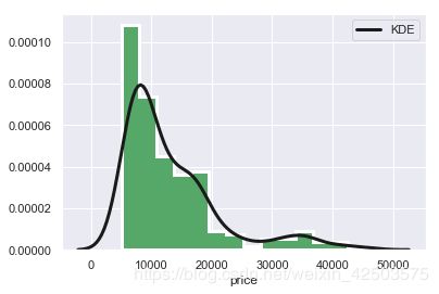
# 分析汽车价格的分布是否符合正态
# data['price'] = np.log(data['price'])
x = data['price']
sns.distplot(x, hist=True, kde=True, kde_kws={"color": "k", "lw": 3, "label": "KDE"},
                   hist_kws={"histtype": "stepfilled", "linewidth": 3,
                             "alpha": 1, "color": "g"})
# 认为基本满足,但有点儿偏态分布了,可以需要通过其他的方式进行加工处理。
数据预处理
特征融合
# 数据预处理
data2 = data.copy()
data2['volume'] = data2.length * data2.width * data2.height
#drop默认删除行元素,删除列需加 axis = 1
data2.drop(['width', 'length', 'height',
           'curb-weight', 'city-mpg'],
          axis = 1, # 1 for columns
          inplace = True)
数值型特征的标准化
# 提取预测值
target = data2['price']
target = data2.price

# 剔除预测值后的其他变量
features = data2.drop(columns=['price'])
# 取数字值有
num = ['symboling', 'normalized-losses', 'volume', 'horsepower', 'wheel-base',
       'bore', 'stroke','compression-ratio', 'peak-rpm','engine-size','highway-mpg']
standard_scaler = StandardScaler()
features[num] = standard_scaler.fit_transform(features[num])
features.head(10)
# 绘制箱线图看数据分布() 但由于数据的度量范围不一致,差距比较大,应在进行归一化后再识别
# https://cloud.tencent.com/developer/article/1441795(如何解决标签重叠的问题)
# plt.figure(figsize = (100, 50)) 试图通过拉长画布解决,但在标签很多的情况下,还是无法实现
features.plot.box(title="Auto-Car", vert=False)
plt.xticks(rotation=-20)

plt.figure()
sns.boxplot(data=features, linewidth=2.5, orient='h')


类别数据编码
# 类别属性的独热编码
classes = ['make', 'fuel-type', 'aspiration', 'num-of-doors',
           'body-style', 'drive-wheels', 'engine-location',
           'engine-type', 'num-of-cylinders', 'fuel-system']
# 将数据转化成独热编码, 即對非數值類型的字符進行分類轉換成數字。用0-1表示,这就将许多指标划分成若干子列,因此现在总共是66列
dummies = pd.get_dummies(features[classes])
#将分类处理后的数据列添加进列表中同时删除处理前的列
# 采用这种方式的好处:每列的名称不是无意义的
features3 = features.join(dummies).drop(classes, axis = 1)
print(features.columns)
# one_hot_encoder = OneHotEncoder()
# # 小心,有两组数据不用进行标准化
# features3 = pd.concat([features[num],pd.DataFrame(one_hot_encoder.fit_transform(features[classes]).toarray())], axis=1)
features3.head()
Index(['symboling', 'normalized-losses', 'make', 'fuel-type', 'aspiration',
       'num-of-doors', 'body-style', 'drive-wheels', 'engine-location',
       'wheel-base', 'engine-type', 'num-of-cylinders', 'engine-size',
       'fuel-system', 'bore', 'stroke', 'compression-ratio', 'horsepower',
       'peak-rpm', 'highway-mpg', 'volume'],
      dtype='object')
数据建模
划分数据集
# sklearn.model_selection.train_test_split随机划分训练集和测试集
X_train, X_test, y_train, y_test = train_test_split(features3, target,
                                                    test_size = 0.3,
                                                    random_state = seed)
模型调参
相关运行中参数的可视化输出
方法一:建一個for循环
alphas = 2. ** np.arange(2, 12)     #array([2,3,4,5,6,7,8,9,10,11])
scores = np.empty_like(alphas)
c = '#366DE8'
#用不同的alphas值做模型
for i, a in enumerate(alphas):  #i:alphas索引序列,a:alphas
    lasso = Lasso(random_state = seed)  #指定lasso模型
    lasso.set_params(alpha = a)  #确定alpha值
    lasso.fit(X_train, y_train) #.fit(x,y) 执行
    scores[i] = lasso.score(X_test, y_test)  #用测试值计算
方法二:常用交叉验证
#lassocv:交叉验证模型,
#lassocv返回拟合优度这一统计学指标,越趋近1,拟合程度越好
lassocv = LassoCV(cv = 10, random_state=seed)#制定模型,将训练集平均切10分,9份用来做训练,1份用来做验证,可设置alphas=[]是多少(序列格式),默认不设置则找适合训练集最优alpha
lassocv.fit(features3, target)  #输入数据训练训练模型
lassocv_score = lassocv.score(features3, target)  #测试模型,返回r^2
lassocv_alpha = lassocv.alpha_   #即确定出最佳惩罚系数 入

plt.figure(figsize = (10, 4))
plt.plot(alphas, scores, '-ko')
#在图上添加一条水平线
plt.axhline(lassocv_score, color = c)
plt.xlabel(r'$\alpha$')
plt.ylabel('CV Score')
plt.xscale('log', basex = 2)
#两个坐标轴与图像的偏移距离
sns.despine(offset = 15)

print('CV results:', lassocv_score, lassocv_alpha)
模型训练
# 看一下权重的分布
# lassocv 回归系数   lassocv.coef_是参数向量w
#pd.Series(data,index)
coefs = pd.Series(lassocv.coef_, index = features3.columns)  # .coef_ 可以返回经过学习后的所有 feature 的参数。

# prints out the number of picked/eliminated features
print("Lasso picked " + str(sum(coefs != 0)) + " features and eliminated the other " +  \
      str(sum(coefs == 0)) + " features.")
#在汽车价格预测中,最重要的正向 feature 是 volume,这个比较贴近现实
# takes first and last 10
coefs = pd.concat([coefs.sort_values().head(5), coefs.sort_values().tail(5)])   #将相同字段首尾相接

plt.figure(figsize = (10, 4))
coefs.plot(kind = "barh", color = c)
# sns.barplot(data=coefs)
plt.title("Coefficients in the Lasso Model")
plt.show()

模型测试
# 测试集
model_l1 = LassoCV(alphas=alphas, cv=10, random_state=seed).fit(X_train, y_train)
y_pred_l1 = model_l1.predict(X_test)

model_l1.score(X_test, y_test)
0.8302697453896324
# residual plot
plt.rcParams['figure.figsize'] = (6.0, 6.0)

preds = pd.DataFrame({"preds": model_l1.predict(X_train), "true": y_train})
preds["residuals"] = preds["true"] - preds["preds"]
sns.scatterplot(x='preds',y="residuals",data=preds)

print(mean_squared_error(y_test, y_pred_l1), r2_score(y_test, y_pred_l1))
3935577.218151757 0.8302697453896325
# 预测结果与实际结果对照
d = {'true' : y_test,
     'predicted' : y_pred_l1
    }

pd.DataFrame(d).head()
模型应用
给定未知数据并输出
如同模型测试中的方法一致,使用predict方法