13 Python总结之估值

未定权益的估值

蒙特卡洛模拟的最重要应用之一是未定权益（期权，衍生品，混合型工具等）的估值。简单地说，在风险中立的世界中，未定权益的价值是风险中立（鞅）测度下的折现后预期收益。这是所有风险因素（股票、指数等）偏离无风险短期利率的概率测度。根据资产定价基本定理，这种概率测度的存在等价于套利机会的缺失。

金融期权表示在规定（行权期）日期（欧式期权）或者规定时期（美式期权）内，以规定价格（所谓行权价 ） 购买（看涨期权 ） 或者出售（看跌期权）指定金融工具。我们首先考虑估值较为简单的情况一欧式期权。

1 欧式期权

基于某种指数的欧式看涨期权到期日收益通过公式h(ST)≡max(ST−K,0)h(ST)≡max(ST−K,0) 得出，其中 STST 是到期日 T 的指数水平，K 是行权价格。给定相关随机过程（例如 几何布朗运动）的风险中立测度，或者在一个完备市场中，这种权证的价格由下面公式表示。

公式 风险中立预期定价

下面公式提供了欧式期权的对应蒙特卡洛模拟公式，其中SiT~ 是到期日期的第 i 个模拟指数水平。

公式 风险中立蒙特卡洛模拟公式

现在考虑几何布朗运动的参数化和估值函数gbm_mcs＿stat， 该函数仅以行权价格作为参数。 这里只模拟到期日的指数水平：

import numpy as np
import numpy.random as random
import matplotlib.pyplot as plt

S0 = 100.
r = 0.05
sigma = 0.25
T = 1.0
I = 50000

# 生成用于过程模拟的标准正态随机数
def gen_sn(M, I, anti_paths=True, mo_math=True):
    """
    Function to generate random numbers for simulation
    :param M: number of time  intervals for discretization
    :param I: number of paths to be simulated
    :param anti_paths: use of antithetic variates
    :param mo_math: use of moment matching
    :return:
    """
    if anti_paths is True:
        sn = random.standard_normal((M + 1, int(I / 2)))
        sn = np.concatenate((sn, -sn), axis=1)
    else:
        sn = random.standard_normal((M + 1, I))
    if mo_math is True:
        sn = (sn - sn.mean()) / sn.std()
    return sn

def gbm_mcs_stat(K):
    """
    Valuation of European call option in Black-Scholes-Merton
    by Mont Carlo simulation ( of index level at maturity )
    :param k: float (positive) strike price of the option
    :return:
    """
    sn = gen_sn(1, I)
    # simulate index level at maturity
    ST = S0 * np.exp((r - 0.5 * sigma ** 2) * T + sigma * np.sqrt(T) * sn[1])
    # calculate payoff at maturity
    hT = np.maximum(ST - K, 0)
    # calculate MCS estimator
    C0 = np.exp(-r * T) * 1 / I * np.sum(hT)
    return C0

作为参考 ， 考虑行权价K=105的情况：

gbm_mcs_stat(K=105.)

9.934031906470926

接下来 ， 我们考虑动态模拟方法 ， 除了看涨期权之外还可以模拟欧式看跌期权。 函数gbm_mcs_dyna 实现了这一算法：

M = 50


def gbm_mcs_dyna(K, option='call'):
    """
    Valuation of European option in Black-Scholes-Merton by Monte Carlo simulation(of index level paths)
    :param K: （positive）strike price of the option
    :param option:
    :return:
    """
    dt = T / M
    # simulation of index level paths
    S = np.zeros((M + 1, I))
    S[0] = S0
    sn = gen_sn(M, I)
    for t in range(1, M + 1):
        S[t] = S[t - 1] * np.exp((r - 0.5 * sigma ** 2) * dt + sigma * np.sqrt(dt) * sn[t])
    # case-based calculation of payoff
    if option == 'call':
        hT = np.maximum(S[-1] - K, 0)
    else:
        hT = np.maximum(K - S[-1], 0)
    # calculation of MCS estimator
    C0 = np.exp(-r * T) * 1 / I * np.sum(hT)
    return C0

12.671844318892582

现在，可以比较相同行权价的看涨和看跌期权的价格估算：

gbm_mcs_dyna(K=110.,option='call')

8.042957534549014

gbm_mcs_dyna(K=110.,option='put')

12.653996825176034

问题是，这些基于模拟的估值方法与Black-Scholes-Merton 估值公式得出的基准值相比表现如何？为了找出这种差别，我们用BSM_Flncrions.py摸块中的Black-Scholes-Metron 分析性欧式看涨期权定价公式生成一定范围行权价的对应期权价值/估值：

def bsm_call_value(S0, K, T, r, sigma):
    ''' Valuation of European call option in BSM model.
    Analytical formula.
    
    Parameters
    ==========
    S0 : float
        initial stock/index level
    K : float
        strike price
    T : float
        maturity date (in year fractions)
    r : float
        constant risk-free short rate
    sigma : float
        volatility factor in diffusion term
    
    Returns
    =======
    value : float
        present value of the European call option
    '''
    from math import log, sqrt, exp
    from scipy import stats

    S0 = float(S0)
    d1 = (log(S0 / K) + (r + 0.5 * sigma ** 2) * T) / (sigma * sqrt(T))
    d2 = (log(S0 / K) + (r - 0.5 * sigma ** 2) * T) / (sigma * sqrt(T))
    value = (S0 * stats.norm.cdf(d1, 0.0, 1.0)
            - K * exp(-r * T) * stats.norm.cdf(d2, 0.0, 1.0))
      # stats.norm.cdf --> cumulative distribution function
      #                    for normal distribution
    return value

# Vega function

stat_res=[]
dyna_res=[]
anal_res=[]
k_list=np.arange(80.,120.1,5.)
np.random.seed(200000)
for K in k_list:
    stat_res.append(gbm_mcs_stat(K))
    dyna_res.append(gbm_mcs_dyna(K))
    anal_res.append(bsm_call_value(S0,K,T,r,sigma))

stat_res = np.array(stat_res)
dyna_res = np.array(dyna_res)
anal_res = np.array(anal_res)

# 首先，我们将静态模拟方法的结果与精确的分析值相比;
fig,(ax1,ax2)= plt.subplots(2,1,sharex=True,figsize=(8,6))
ax1.plot(k_list,anal_res,'b',label='analytical')
ax1.plot(k_list,stat_res,'ro',label='static')
ax1.set_ylabel('European call option value')
ax1.grid(True)
ax1.legend(loc=0)
ax1.set_ylim(ymin=0)
wi=1.0
ax2.bar(k_list-wi/2,(np.array(anal_res)-np.array(stat_res))/np.array(anal_res)*100,wi)
ax2.set_xlabel('strike')
ax2.set_ylabel('difference in %')
ax2.set_xlim(left=75,right=125)
ax2.grid(True)

合并动态模拟和估值方法的类似图表， 可以得到下图的结果。同样，所有估值差异小于1% ， 标准差既有负数也有正数的情况。作为一般原则 ， 蒙特卡洛估算函数的质量可以通过调整使用的时间间隔 M 和模拟路径数 I 控制。

fig,(ax1,ax2)= plt.subplots(2,1,sharex=True,figsize=(8,6))
ax1.plot(k_list,anal_res,'b',label='analytical')
ax1.plot(k_list,dyna_res,'ro',label='dynamic')
ax1.set_ylabel('European call option value')
ax1.grid(True)
ax1.legend(loc=0)
ax1.set_ylim(ymin=0)
wi=1.0
ax2.bar(k_list-wi/2,(np.array(anal_res)-np.array(dyna_res))/np.array(anal_res)*100,wi)
ax2.set_xlabel('strike')
ax2.set_ylabel('difference in %')
ax2.set_xlim(left=75,right=125)
ax2.grid(True)

2 美式期权

美式期权的估值比欧式期权更复杂。在这种情况下， 必须解决最优截止问题，提出期权的公允价值。下面公式是将美式期权作为最优截止问题时的估值公式。该问题的公式化已经基于离散的时间网络， 以便用于数值化模拟。 在某种意义上， 更准确地说，这是百慕大式期权的估值公式。 时间间隔收敛干0长度时， 百慕大期权的价值收敛于美式期权的价值。

公式 以最优截止问题形式出现的美式期权价格：

下面描述的算法称为最小二乘蒙特卡洛（LSM）方法。由Vt(s)=max(ht(s),Ct(s))Vt(s)=max(ht(s),Ct(s)) (其中Ct(s)=EQt(e−rΔtVt+Δt(St+Δt)|St=s)Ct(s)=EtQ(e−rΔtVt+Δt(St+Δt)|St=s) ) 给出的任何给定日期 t 的美式（百慕大）期权价值是给定指数水平 St=sSt=s 下的期权持续价值。
现在我们考虑在 M 个等长 （ΔtΔt）的时间间隔中模拟指数水平的 I 条路径。 定义 Yt,i≡e−rΔtVt+Δt,iYt,i≡e−rΔtVt+Δt,i 为路径 i 在时间 t 时的模拟持续价值。我们不能直接使用这个数字，因为它意味着完美的预期。但是，我们可以使用所有模拟持续价值的截面，通过最下二乘回归估算（预期）持续价值。

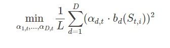
给定一组基函数 bd,d=1,…,Dbd,d=1,…,D , 然后由回归估算公式 C^{t,i=∑Dd=1α∗d,t⋅bd(St,i)C}t,i=∑d=1Dαd,t∗⋅bd(St,i) 算出持续价值，其中最优回归参数 α∗α∗ 是下面公式中最小二乘法问题的解。

公式 美式期权估值的最小二乘回归:

gbm_mcs_amer 函数实现美式看涨和看跌期权的LSM 算法：

def gbm_mcs_amer(K, option='call'):
    """
    Valuation of American option in Black-Scholes-Merton
    by Monte Carlo simulation by LSM algorithm
    :param K: (positive) strike price of the option
    :param option: type of the option to be valued ('call','put')
    :return: estimated present value of American call option
    """
    dt = T / M
    df = np.exp(-r * dt)
    # simulation of index levels
    S = np.zeros((M + 1, I))
    S[0] = S0
    sn = gen_sn(M, I)
    for t in range(1, M + 1):
        S[t] = S[t - 1] * np.exp((r - 0.5 * sigma ** 2) * dt
                                 + sigma * np.sqrt(dt) * sn[t])
    # case-based calculation of payoff
    if option == 'call':
        h = np.maximum(S - K, 0)
    else:
        h = np.maximum(K - S, 0)
    # LSM algorithm
    V = np.copy(h)
    for t in range(M - 1, 0, -1):
        reg = np.polyfit(S[t], V[t + 1] * df, 7)
        C = np.polyval(reg, S[t])
        V[t] = np.where(C > h[t], V[t + 1] * df, h[t])
    # MSC estimator
    C0 = df * 1 / I * np.sum(V[1])
    return C0

gbm_mcs_amer(110.,option='call')

7.796943788560202

gbm_mcs_amer(110.,option='put')

13.660914609034444

欧式期权的价值处于美式期权价值的下界。 两者的差异通常称作提前行权溢价。 下面，我们比较和以前相同的行权价范围内的欧式和美式期权价值， 以估算期权溢价。 这次我们选择看跌期权：

euro_res = []
amer_res =[]
k_list = np.arange(80., 120.1, 5.)
for K in k_list:
    euro_res.append(gbm_mcs_dyna(K,'put'))
    amer_res.append(gbm_mcs_amer(K,'put'))
euro_res = np.array(euro_res)
amer_res = np.array(amer_res)

下图说明对于所选择的行权价范围，溢价可能最高达到10%

fig, (ax1 ,ax2) = plt.subplots(2, 1, sharex=True, figsize=(8, 6))
ax1. plot(k_list, euro_res,'b', label='European put')
ax1. plot(k_list, amer_res,'ro',label='American put')
ax1.set_ylabel('call option value')
ax1.grid(True)
ax1.legend(loc=0)
wi = 1.0
ax2.bar(k_list - wi / 2, (amer_res - euro_res) / euro_res * 100, wi)
ax2.set_xlabel('strike')
ax2.set_ylabel('early exercise premium in %')
ax2.set_xlim(left=75, right=125)
ax2.grid(True)

欧式期权和LSM蒙特卡洛估算值的对比