tensorflow2.x第二篇
学习率策略,激活函数,正态分布函数,tf.where,正则化,交叉熵损失函数,优化参数策略
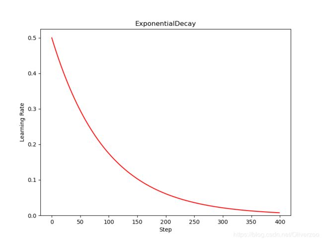
- 指数衰减学习率策略
import tensorflow as tf
import matplotlib.pyplot as plt
N = 400
'''
tf.keras.optimizers.schedules.ExponentialDecay(
        initial_learning_rate,
        decay_steps,
        decay_rate,
        staircase=False,
        name=None )
initial_learning_rate: 初始学习率.
decay_steps: 衰减步数, staircase为True时有效.
decay_rate: 衰减率.
staircase: Bool型变量.如果为True, 学习率呈现阶梯型下降趋势
***************************************************
lr = LR_BASE*LR_DECAY**(epoch/LR_STEP)
'''
lr_shedule = tf.keras.optimizers.schedules.ExponentialDecay(
    0.5,
    decay_steps=10,
    decay_rate=0.9,
    staircase=True
)
y = []
for global_step in range(N):
    lr = lr_shedule(global_step)
    y.append(lr)
x = range(N)
plt.figure(figsize=(8,6))
plt.plot(x,y,'r-')
plt.ylim([0,max(plt.ylim())])
plt.xlabel('Step')
plt.ylabel('Learning Rate')
plt.title('ExponentialDecay')
plt.show()

实例:
import tensorflow as tf

w = tf.Variable(tf.constant(5.,tf.float32))
epoch = 40
LR_BASE = 0.2  # 最初学习率
LR_DECAY = 0.99  # 学习率衰减率
LR_STEP = 1  # 喂入多少轮BATCH_SIZE后,更新一次学习率

for epoch in range(epoch):
    lr = LR_BASE*LR_DECAY**(epoch/LR_STEP)
    with tf.GradientTape() as tape:
        loss = tf.square(w-3)
    grads = tape.gradient(loss,w)
    w.assign_sub(lr*grads)
    print("After %s epoch,w is %f,loss is %f,lr is %f" % (epoch, w.numpy(), loss, lr))
out:
After 32 epoch,w is 3.000002,loss is 0.000000,lr is 0.144996
After 33 epoch,w is 3.000001,loss is 0.000000,lr is 0.143546
After 34 epoch,w is 3.000001,loss is 0.000000,lr is 0.142111
After 35 epoch,w is 3.000001,loss is 0.000000,lr is 0.140690
After 36 epoch,w is 3.000000,loss is 0.000000,lr is 0.139283
After 37 epoch,w is 3.000000,loss is 0.000000,lr is 0.137890
After 38 epoch,w is 3.000000,loss is 0.000000,lr is 0.136511
After 39 epoch,w is 3.000000,loss is 0.000000,lr is 0.135146

Process finished with exit code 0
- 分段常数衰减学习率策略
import tensorflow as tf
import matplotlib.pyplot as plt
N = 400
'''
tf.keras.optimizers.schedules.PiecewiseConstantDecay(
            boundaries,
            values,
            name=None )
boundaries: [step_1, step_2, ..., step_n]定义了在第几步进行学习率衰减.
values: [val_0, val_1, val_2, ..., val_n]定义了学习率的初始值和后续衰减时的具体取值.
'''
lr_schedule = tf.keras.optimizers.schedules.PiecewiseConstantDecay(
    boundaries = [100,200,300],
    values = [0.1,0.05,0.025,0.001]
)
y = []
for global_step in range(N):
    lr = lr_schedule(global_step)
    y.append(lr)
x = range(N)
plt.figure(figsize=(8,6))
plt.plot(x,y,'r-')
plt.ylim([0,max(plt.ylim())])
plt.xlabel('Step')
plt.ylabel('Learning Rate')
plt.title('PiecewiseConstantDecay')
plt.show()

- 关于激活函数
1.sigmoid:多用于二分类
2.tanh:很大程度上优于sigmoid
3.relu:多分类卷积神经网络用
4.softmax:转化概率
****多用rulu
****输入标准化(输入特征标准化,即让输入特征满足以0为均值,1为标准差的正态分布;)
****初始化:零均值,sqrt(2/当前层特征数)为标准差的正态分布
体会soft作用
import tensorflow as tf
import numpy as np

y_ = np.array([[1, 0, 0], [0, 1, 0], [0, 0, 1], [1, 0, 0], [0, 1, 0]])
y = np.array([[12, 3, 2], [3, 10, 1], [1, 2, 5], [4, 6.5, 1.2], [3, 6, 1]])
y_pred = tf.nn.softmax(y)
print(y_pred)
loss_ce1 = tf.losses.categorical_crossentropy(y_,y_pred)
loss_ce2 = tf.nn.softmax_cross_entropy_with_logits(y_,y)

print('分步计算的结果:\n', loss_ce1)
print('结合计算的结果:\n', loss_ce2)
out:
分步计算的结果:
 tf.Tensor(
[1.68795487e-04 1.03475622e-03 6.58839038e-02 2.58349207e+00
 5.49852354e-02], shape=(5,), dtype=float64)
结合计算的结果:
 tf.Tensor(
[1.68795487e-04 1.03475622e-03 6.58839038e-02 2.58349207e+00
 5.49852354e-02], shape=(5,), dtype=float64)

Process finished with exit code 0
- 交叉熵损失函数辨析
import tensorflow as tf
'''
tf.keras.losses.categorical_crossentropy(
        y_true,
        y_pred,
        from_logits=False,
        label_smoothing=0 )
y_true: 真实值.
y_pred: 预测值.
from_logits: y_pred是否为logits张量.
label_smoothing: [0,1]之间的小数.

在机器学习中,对于多分类问题,把未经softmax归一化的向量值称为logits。logits经过softmax
层后,输出服从概率分布的向量。
'''
y_true = [1,0,0]
y_pred1 = [0.5,0.4,0.1]
y_pred2 = [0.8,0.1,0.1]
print(tf.keras.losses.categorical_crossentropy(y_true,y_pred1))
print(tf.keras.losses.categorical_crossentropy(y_true,y_pred2))

#等价
print(-tf.reduce_sum(y_true*tf.math.log(y_pred1)))
print(-tf.reduce_sum(y_true*tf.math.log(y_pred2)))
out:
tf.Tensor(0.6931472, shape=(), dtype=float32)
tf.Tensor(0.22314353, shape=(), dtype=float32)
tf.Tensor(0.6931472, shape=(), dtype=float32)
tf.Tensor(0.22314353, shape=(), dtype=float32)
import tensorflow as tf
'''
tf.nn.softmax_cross_entropy_with_logits(
            labels,
            logits,
            axis=-1,
            name=None )
labels: 在类别这一维度上,每个向量应服从有效的概率分布.
        例如,在labels的shape为[batch_size, num_classes]的情况下,labels[i]应服从概率分布.
logits: 每个类别的激活值,通常是线性层的输出. 激活值需要经过softmax归一化.
axis: 类别所在维度,默认是-1,即最后一个维度.
'''
labels = [[1.0, 0.0, 0.0], [0.0, 1.0, 0.0]]
logits = [[4.0, 2.0, 1.0], [0.0, 5.0, 1.0]]
print(tf.nn.softmax_cross_entropy_with_logits(labels=labels,logits=logits))

#等价
print(-tf.reduce_sum(labels*tf.math.log(tf.nn.softmax(logits)),axis=1))
out:
tf.Tensor([0.16984604 0.02474492], shape=(2,), dtype=float32)
tf.Tensor([0.16984606 0.02474495], shape=(2,), dtype=float32)
import tensorflow as tf
'''
tf.nn.sparse_softmax_cross_entropy_with_logits(
            labels,
            logits,
            name=None )
labels经过one-hot编码,logits经过softmax,两者进行交叉熵计算. 通常
labels的shape为[batch_size],logits的shape为[batch_size, num_classes].
******sparse可理解为对labels进行稀疏化处理(即进行one-hot编码)

labels: 标签的索引值.
logits: 每个类别的激活值,通常是线性层的输出. 激活值需要经过softmax归一化.
'''
labels = [0,1]
logits = [[4.0,2.0,1.0],[0.0,5.0,1.0]]
print(tf.nn.sparse_softmax_cross_entropy_with_logits(labels,logits))

#等价
print(-tf.reduce_sum(tf.one_hot(labels,tf.shape(logits)[1])*tf.math.log(tf.nn.softmax(logits)),axis=1))
out:
tf.Tensor([0.16984604 0.02474492], shape=(2,), dtype=float32)
tf.Tensor([0.16984606 0.02474495], shape=(2,), dtype=float32)
- 正态分布函数
import tensorflow as tf
'''
tf.random.normal(
            shape,
            mean=0.0,
            stddev=1.0,
            dtype=tf.dtypes.float32,
            seed=None,
            name=None )
x: 一维张量.
mean: 正态分布的均值.
stddev: 正态分布的方差.
'''
print(tf.random.normal([2,2],mean=0.0,stddev=1.0))
out:
tf.Tensor(
[[ 1.2957982 -0.573582 ]
 [ 1.3670938  2.0009952]], shape=(2, 2), dtype=float32)
- tf.where
import tensorflow as tf
'''
tf.where( condition, x=None, y=None, name=None )

根据condition,取x或y中的值。如果为True,对应位置取x的值;如果为
False,对应位置取y的值。
'''
a = tf.constant([1, 2, 3, 1, 1])
b = tf.constant([0, 1, 3, 4, 5])
c = tf.where(tf.greater(a,b),a,b)
print(c)
out:
tf.Tensor([1 2 3 4 5], shape=(5,), dtype=int32)
-
过拟合和欠拟合
欠拟合的解决方法:增加输入特征项 增加网络参数 减少正则化参数
过拟合的解决方法:
		数据清洗
		增大训练集
		采用正则化
		增大正则化参数
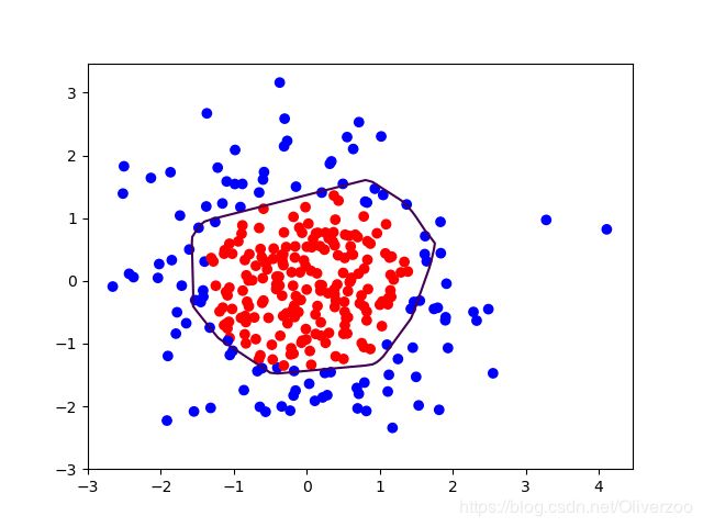
正则化:
# 导入所需模块
import tensorflow as tf
from matplotlib import pyplot as plt
import numpy as np
import pandas as pd
# 读入数据/标签 生成x_train y_train
df = pd.read_csv('dot.csv')
x_data = np.array(df[['x1', 'x2']])
y_data = np.array(df['y_c'])
x_train = np.vstack(x_data).reshape(-1, 2)
y_train = np.vstack(y_data).reshape(-1, 1)
Y_c = [['red' if y else 'blue'] for y in y_train]
# 转换x的数据类型,否则后面矩阵相乘时会因数据类型问题报错
x_train = tf.cast(x_train, tf.float32)
y_train = tf.cast(y_train, tf.float32)
# from_tensor_slices函数切分传入的张量的第一个维度,生成相应的数据集,使输入特征和标签值一一对应
train_db = tf.data.Dataset.from_tensor_slices((x_train, y_train)).batch(32)
# 生成神经网络的参数,输入层为2个神经元,隐藏层为11个神经元,1层隐藏层,输出层为1个神经元
# 用tf.Variable()保证参数可训练
w1 = tf.Variable(tf.random.normal([2, 11]), dtype=tf.float32)
b1 = tf.Variable(tf.constant(0.01, shape=[11]))
w2 = tf.Variable(tf.random.normal([11, 1]), dtype=tf.float32)
b2 = tf.Variable(tf.constant(0.01, shape=[1]))
lr = 0.005 # 学习率
epoch = 800 # 循环轮数
# 训练部分
for epoch in range(epoch):
for step, (x_train, y_train) in enumerate(train_db):
with tf.GradientTape() as tape: # 记录梯度信息
h1 = tf.matmul(x_train, w1) + b1 # 记录神经网络乘加运算
h1 = tf.nn.relu(h1)
y = tf.matmul(h1, w2) + b2
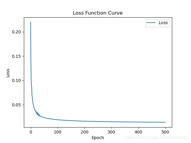
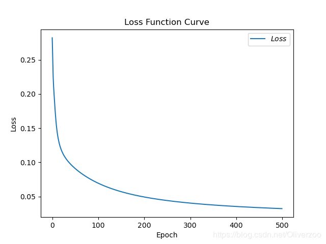
# 采用均方误差损失函数mse = mean(sum(y-out)^2)
loss = tf.reduce_mean(tf.square(y_train - y))
'''
#++++++++++++++++++++++++++++++++++
#在这里添加正则化项
loss_regularization = []
loss_regularization.append(tf.nn.l2_loss(w1))
loss_regularization.append(tf.nn.l2_loss(w2))
loss_regularization = tf.reduce_sum(loss_regularization)
loss = loss_mse + 0.03 * loss_regularization
'''
# 计算loss对各个参数的梯度
variables = [w1, b1, w2, b2]
grads = tape.gradient(loss, variables)
# 实现梯度更新
# w1 = w1 - lr * w1_grad tape.gradient是自动求导结果与[w1, b1, w2, b2] 索引为0,1,2,3
w1.assign_sub(lr * grads[0])
b1.assign_sub(lr * grads[1])
w2.assign_sub(lr * grads[2])
b2.assign_sub(lr * grads[3])
# 每20个epoch,打印loss信息
if epoch % 20 == 0:
print('epoch:', epoch, 'loss:', float(loss))
# 预测部分
print("*******predict*******")
# xx在-3到3之间以步长为0.01,yy在-3到3之间以步长0.01,生成间隔数值点
xx, yy = np.mgrid[-3:3:.1, -3:3:.1]
# 将xx , yy拉直,并合并配对为二维张量,生成二维坐标点
grid = np.c_[xx.ravel(), yy.ravel()]
grid = tf.cast(grid, tf.float32)
# 将网格坐标点喂入神经网络,进行预测,probs为输出
probs = []
for x_test in grid:
# 使用训练好的参数进行预测
h1 = tf.matmul([x_test], w1) + b1
h1 = tf.nn.relu(h1)
y = tf.matmul(h1, w2) + b2 # y为预测结果
probs.append(y)
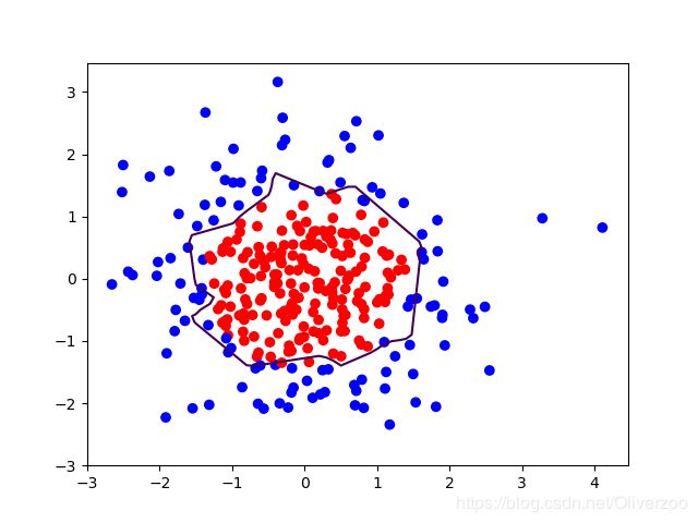
# 取第0列给x1,取第1列给x2
x1 = x_data[:, 0]
x2 = x_data[:, 1]
# probs的shape调整成xx的样子
probs = np.array(probs).reshape(xx.shape)
plt.scatter(x1, x2, color=np.squeeze(Y_c)) # squeeze去掉纬度是1的纬度,相当于去掉[['red'],[''blue]],内层括号变为['red','blue']
# 把坐标xx yy和对应的值probs放入contour函数,给probs值为0.5的所有点上色 plt.show()后 显示的是红蓝点的分界线
plt.contour(xx, yy, probs, levels=[.5])
plt.show()
# 读入红蓝点,画出分割线,不包含正则化
# 不清楚的数据,建议print出来查看
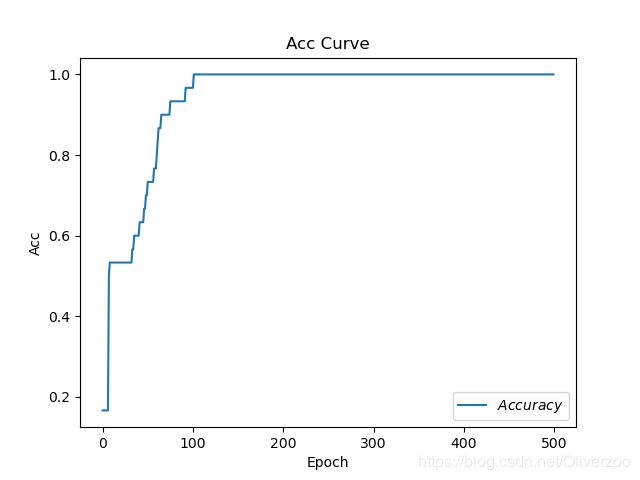
- 几种优化器辨析
SGD:
下降速度慢,而且可能会在沟壑的两边持续震荡,停留在一个局部最优点
# sgd
w1.assign_sub(learning_rate * grads[0])
b1.assign_sub(learning_rate * grads[1])
total_time 9.204401731491089
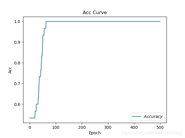
SGD with Momentum:
动量法是一种使梯度向量向相关方向加速变化,抑制震荡,最终实现加速收敛的方法
#sgd-momentun
beta = 0.9
m_w = beta * m_w + (1 - beta) * grads[0]
m_b = beta * m_b + (1 - beta) * grads[1]
w1.assign_sub(learning_rate * m_w)
b1.assign_sub(learning_rate * m_b)
total_time 11.45138669013977
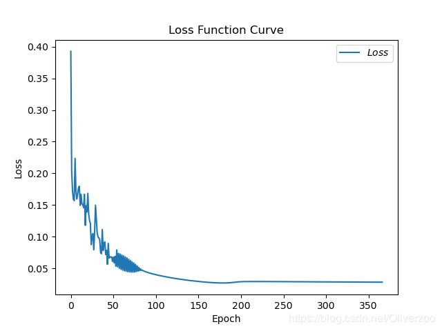
SGD所有参数共享一个学习率,不同参数的更新能力不同,那么我们给它们适合自己的学习率,这一过程如何实现?一阶导数代表参数更新最快的方向,一阶导数的平方的和就表示该参数的更新能力。由此引入AdaGrad(学习率衰减过快?)
# adagrad
v_w += tf.square(grads[0])
v_b += tf.square(grads[1])
w1.assign_sub(learning_rate * grads[0] / tf.sqrt(v_w))
b1.assign_sub(learning_rate * grads[1] / tf.sqrt(v_b))
total_time 10.391653537750244

然后为了减慢学习率的衰减:RMSProp
beta = 0.9
v_w = beta * v_w + (1 - beta) * tf.square(grads[0])
v_b = beta * v_b + (1 - beta) * tf.square(grads[1])
w1.assign_sub(learning_rate * grads[0] / tf.sqrt(v_w))
b1.assign_sub(learning_rate * grads[1] / tf.sqrt(v_b))
total_time 11.450389623641968
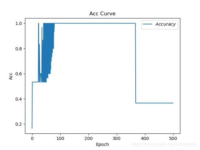
最后Adam把上面所有的优点集中
m_w = beta1 * m_w + (1 - beta1) * grads[0]
m_b = beta1 * m_b + (1 - beta1) * grads[1]

v_w = beta2 * v_w + (1 - beta2) * tf.square(grads[0])
v_b = beta2 * v_b + (1 - beta2) * tf.square(grads[1])

m_w_correction = m_w / (1 - tf.pow(beta1, int(global_step)))
m_b_correction = m_b / (1 - tf.pow(beta1, int(global_step)))
v_w_correction = v_w / (1 - tf.pow(beta2, int(global_step)))
v_b_correction = v_b / (1 - tf.pow(beta2, int(global_step)))

w1.assign_sub(learning_rate * m_w_correction / tf.sqrt(v_w_correction)) b1.assign_sub(learning_rate * m_b_correction / tf.sqrt(v_b_correction))
total_time 16.22359299659729