机器学习网格搜索寻找最优参数

整理一下前阶段复习的关于网格搜索的知识：

程序及数据 请到github 上 下载 GridSearch练习

网格搜索是将训练集训练的一堆模型中，选取超参数的所有值（或者代表性的几个值），将这些选取的参数及值全部列出一个表格，并分别将其进行模拟，选出最优模型。

上面是数据集的可视化分布图，具体代码如下：

%matplotlib inline
import pandas as pd
import numpy as np
import matplotlib.pyplot as plt

data = pd.read_csv('data/grid.csv',header=None)
X = data[[0,1]]
y = data[2]
#print(y)
X_blue = data[data[2]== 0]
X_red = data[data[2]== 1]
plt.scatter(X_blue[0],X_blue[1],c='blue',edgecolor='k',s=50)
plt.scatter(X_red[0],X_red[1],c='red',edgecolor='k',s=50)
plt.xlim(-2.05,2.05)
plt.ylim(-2.05,2.05)

采用决策树来训练数据

from sklearn.tree import DecisionTreeClassifier
clf = DecisionTreeClassifier(random_state=42)
clf.fit(X_train,y_train)

train_predictions = clf.predict(X_train)
test_predictions = clf.predict(X_test)
print(clf.get_params())

数据分类可视化自定义函数的代码如下：

def plot_model(X, y, clf):
    plt.scatter(X_blue[0],X_blue[1],c='blue',edgecolor='k',s=50)
    plt.scatter(X_red[0],X_red[1],c='red',edgecolor='k',s=50)

    plt.xlim(-2.05,2.05)
    plt.ylim(-2.05,2.05)
    plt.grid(False)
    plt.tick_params(
        axis='x',
        which='both',
        bottom='off',
        top='off')

    r = np.linspace(-2.1,2.1,300)
    s,t = np.meshgrid(r,r)
    s = np.reshape(s,(np.size(s),1))
    t = np.reshape(t,(np.size(t),1))
    h = np.concatenate((s,t),1)

    z = clf.predict(h)

    s = s.reshape((np.size(r),np.size(r)))
    t = t.reshape((np.size(r),np.size(r)))
    z = z.reshape((np.size(r),np.size(r)))

    plt.contourf(s,t,z,colors = ['blue','red'],alpha = 0.2,levels = range(-1,2))
    if len(np.unique(z)) > 1:
        plt.contour(s,t,z,colors = 'k', linewidths = 2)
    plt.show()

数据集分类的可视化显示：

plot_model(X, y, clf)

 

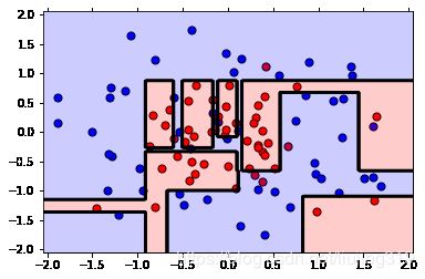
 从上面的界限可视化上来看是处于过拟合的状态，因为在训练数据的时候未设定参数，超参数 max_depth=None 时候，训练数据时候一直到决策树的最底层的叶子节点结束，所以就出现了过拟合的状态。

模型复杂度曲线可视化

from sklearn.model_selection import ShuffleSplit
from sklearn.model_selection import validation_curve
#from sklearn.tree import DecisionTreeRegressor

def ModelComplexity(X, y):
    """ Calculates the performance of the model as model complexity increases.
        The learning and testing errors rates are then plotted. """
    
    # Create 10 cross-validation sets for training and testing
    cv = ShuffleSplit(X.shape[0], test_size = 0.2, random_state = 42)

    # Vary the max_depth parameter from 1 to 10
    max_depth = np.arange(1,11)
    
    scorer = make_scorer(f1_score)

    # Calculate the training and testing scores
    train_scores, test_scores = validation_curve(DecisionTreeClassifier(), X, y, \
        param_name = "max_depth", param_range = max_depth, cv = cv, scoring =scorer)

    # Find the mean and standard deviation for smoothing
    train_mean = np.mean(train_scores, axis=1)
    train_std = np.std(train_scores, axis=1)
    test_mean = np.mean(test_scores, axis=1)
    test_std = np.std(test_scores, axis=1)

    # Plot the validation curve
    plt.figure(figsize=(7, 5))
    plt.title('Decision Tree Classifier Complexity Performance')
    plt.plot(max_depth, train_mean, 'o-', color = 'r', label = 'Training Score')
    plt.plot(max_depth, test_mean, 'o-', color = 'g', label = 'Validation Score')
    plt.fill_between(max_depth, train_mean - train_std, \
        train_mean + train_std, alpha = 0.15, color = 'r')
    plt.fill_between(max_depth, test_mean - test_std, \
        test_mean + test_std, alpha = 0.15, color = 'g')
    
    # Visual aesthetics
    plt.legend(loc = 'lower right')
    plt.xlabel('Maximum Depth')
    plt.ylabel('Score')
    plt.ylim([-0.05,1.05])
    plt.show()

ModelComplexity(X, y)

从上面的复杂度曲线图可以看出，在max_depth=4 的时候 ，训练集和测试集的得分是最接近的，在向右的时候，测试集的得分就呈下降趋势， 虽然此时训练集的得分很高，但训练集的得分下降了，这说明在测试集上模型没有很好的拟合数据，就是过拟合状态了。

下面来采用网格搜索来寻找最优参数，本例中以 max_depth 和min_samples_leaf 这两个参数来进行筛选

from sklearn.model_selection import GridSearchCV
clf = DecisionTreeClassifier(random_state=42)
scorer = make_scorer(f1_score)

parameters = {'max_depth':[2,4,6,8,10],'min_samples_leaf':[2,4,6,8,10], 'min_samples_split':[2,4,6,8,10]}
grid_obj = GridSearchCV(clf, parameters, scoring=scorer)
grid_obj.fit(X_train,y_train)

best_clf = grid_obj.best_estimator_
print(grid_obj.best_params_)

best_clf.fit(X_train,y_train)
best_train_predictions = best_clf.predict(X_train)
best_test_predictions = best_clf.predict(X_test)

print('The training F1 Score is', f1_score(best_train_predictions, y_train))
print('The testing F1 Score is', f1_score(best_test_predictions, y_test))
plot_model(X, y, best_clf)

上面是通过网格搜索得出的最优模型来模拟出来的分类界限可视化图，可以从图中很直观的看出，划分的效果好了很多。

下面看下决策树的分支示意图：图一 是优化前 max_depth=None 的情况，图二 是网格搜索出的最优模型

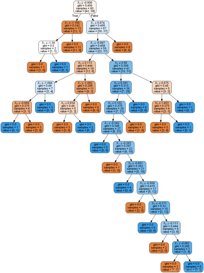
                                                                                                 图1 ：优化前

    

                                                                                图二：网格搜索的最优模型

具体代码在程序中，请大家自行阅读。

最后给出网格搜索前后的模型对比示意图：（学习曲线的可视化程序在github 的源码中，请大家自行下载查看 网格搜索练习）

时间关系，写的比较粗糙，请大家多提宝贵意见，我会逐步改进！