一文搞懂光流 光流的生成，可视化以及映射（backward warp）

本文所有代码公开于github：
https://github.com/weihuang527/optical-flow

什么是光流

官方定义

Optical flow or optic flow is the pattern of apparent motion of objects, surfaces, and edges in a visual scene caused by the relative motion between an observer and a scene. Optical flow can also be defined as the distribution of apparent velocities of movement of brightness pattern in an image. （from 维基百科）

其他解释：
光流是空间运动物体在观察成像平面上的像素运动的瞬时速度，是利用图像序列中像素在时间域上的变化以及相邻帧之间的相关性来找到上一帧跟当前帧之间存在的对应关系，从而计算出相邻帧之间物体的运动信息的一种方法。一般而言，光流是由于场景中前景目标本身的移动、相机的运动，或者两者的共同运动所产生的。(from 博客)

光流表示的是相邻两帧图像中每个像素的运动速度和运动方向。（from 博客）

自己的解释

光流经常出现在视频或图像序列（多张图像）中，用来刻画运动物体（相机或被观察的物体）瞬时的运动转态（运动方向和运动偏移量）

光流的表示

光流的表示也是数字化的。它一般使用一个三维的数组（$[height,width,2]$）表示，其中$height$表示图像的高度，也就是数组中的行数，$width$表示图像的宽度，也就是数组中的列数，$2$表示$x,y$两个方向。

直白地解释：在光流数组的第三维上，第一通道（即$[height,width,0]$）表示图像在$x$方向的偏移方向和大小。这里的$x$方向是水平方向，即图像数组中的行向量方向；
第二通道（即$[height,width,1]$）表示图像在$y$方向的偏移方向和大小。这里的$y$方向是竖直方向，即图像数组中的列向量方向。

这里还要注意的一点：偏移量的大小当然就是通过光流数组中的数值大小体现出来的，而偏移的方向是通过光流数组中的正负体现出来的。在$x$方向上，正值表示物体向左移动，而负值表示物体向右移动；在$y$方向上，正值表示物体向上移动，而负值表示物体向下移动。 至于为什么是这样的，后面我们在backward warp中的源码中进行解释。

光流的生成

光流提取

为了提取光流，一般就需要输入视频中的相邻两帧，或者图像序列中的相邻两张图像，然后通过算法提取出光流。算法包括传统方法也有目前基于深度学习的方法，比如flownet。由于提取光流的算法不是本文的重点，这里就不进行赘述。光流的提取方法也已经有很多优秀的博文进行了介绍，大家可以去参考，这里我也给出一些较优秀博文的链接：
https://zhuanlan.zhihu.com/p/74460341
https://blog.csdn.net/qq_41368247/article/details/82562165
https://my.oschina.net/u/3702502/blog/1815343
https://www.cnblogs.com/sddai/p/10275837.html
https://blog.csdn.net/carson2005/article/details/7581642

生成光流

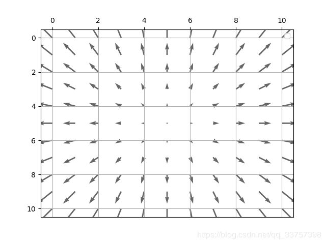
为了能真实感受光流，以及它的格式。这里写了一个小代码来生成一个由一个点向四周扩散的光流，这里的光流数组的shape为$[11,11,2]$，如下图（光流的可视化下面讲解）：

也可以看看这个光流数组里面对应的值到底是什么：

# 第一通道
[[ 2.5  2.   1.5  1.   0.5  0.  -0.5 -1.  -1.5 -2.  -2.5]
 [ 2.5  2.   1.5  1.   0.5  0.  -0.5 -1.  -1.5 -2.  -2.5]
 [ 2.5  2.   1.5  1.   0.5  0.  -0.5 -1.  -1.5 -2.  -2.5]
 [ 2.5  2.   1.5  1.   0.5  0.  -0.5 -1.  -1.5 -2.  -2.5]
 [ 2.5  2.   1.5  1.   0.5  0.  -0.5 -1.  -1.5 -2.  -2.5]
 [ 2.5  2.   1.5  1.   0.5  0.  -0.5 -1.  -1.5 -2.  -2.5]
 [ 2.5  2.   1.5  1.   0.5  0.  -0.5 -1.  -1.5 -2.  -2.5]
 [ 2.5  2.   1.5  1.   0.5  0.  -0.5 -1.  -1.5 -2.  -2.5]
 [ 2.5  2.   1.5  1.   0.5  0.  -0.5 -1.  -1.5 -2.  -2.5]
 [ 2.5  2.   1.5  1.   0.5  0.  -0.5 -1.  -1.5 -2.  -2.5]
 [ 2.5  2.   1.5  1.   0.5  0.  -0.5 -1.  -1.5 -2.  -2.5]]
# 第二通道
[[ 2.5  2.5  2.5  2.5  2.5  2.5  2.5  2.5  2.5  2.5  2.5]
 [ 2.   2.   2.   2.   2.   2.   2.   2.   2.   2.   2. ]
 [ 1.5  1.5  1.5  1.5  1.5  1.5  1.5  1.5  1.5  1.5  1.5]
 [ 1.   1.   1.   1.   1.   1.   1.   1.   1.   1.   1. ]
 [ 0.5  0.5  0.5  0.5  0.5  0.5  0.5  0.5  0.5  0.5  0.5]
 [ 0.   0.   0.   0.   0.   0.   0.   0.   0.   0.   0. ]
 [-0.5 -0.5 -0.5 -0.5 -0.5 -0.5 -0.5 -0.5 -0.5 -0.5 -0.5]
 [-1.  -1.  -1.  -1.  -1.  -1.  -1.  -1.  -1.  -1.  -1. ]
 [-1.5 -1.5 -1.5 -1.5 -1.5 -1.5 -1.5 -1.5 -1.5 -1.5 -1.5]
 [-2.  -2.  -2.  -2.  -2.  -2.  -2.  -2.  -2.  -2.  -2. ]
 [-2.5 -2.5 -2.5 -2.5 -2.5 -2.5 -2.5 -2.5 -2.5 -2.5 -2.5]]

同时再附上生成这个简单光流的代码：

def gen_flow_circle(center, height, width):
    x0, y0 = center
    if x0 >= height or y0 >= width:
        raise AttributeError('ERROR')
    flow = np.zeros((height, width, 2), dtype=np.float32)

    grid_x = np.tile(np.expand_dims(np.arange(width), 0), [height, 1])
    grid_y = np.tile(np.expand_dims(np.arange(height), 1), [1, width])

    grid_x0 = np.tile(np.array([x0]), [height, width])
    grid_y0 = np.tile(np.array([y0]), [height, width])

    flow[:,:,0] = grid_x0 - grid_x
    flow[:,:,1] = grid_y0 - grid_y

    return flow

if __name__ == "__main__":
    # Function: gen_flow_circle
    center = [5, 5]
    flow = gen_flow_circle(center, height=11, width=11)
    flow = flow / 2 # 改变光流的值，也就是改变像素的偏移量，这个不重要

也有其他的光流生成方式：
https://www.cnblogs.com/xianhan/p/10401442.html

光流的可视化

稠密光流可视化

光流的可视化代码摘抄于博客：
https://blog.csdn.net/qq_34535410/article/details/89976801

所以这里就不过多介绍了，能用就行~~
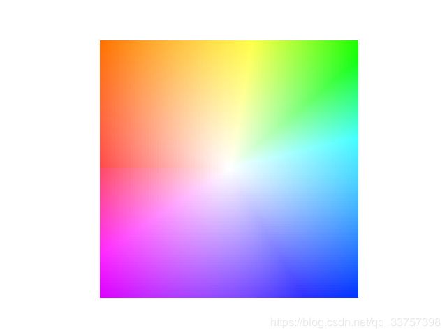
这里只放一个该代码的运行结果，还是上面展示的那个光流，唯一区别就是这里的光流数组大小为$[101,101,2]$， 这个也是Color wheel，它的作用就是给你一个由该代码生成的光流可视化图，你参考这个Color wheel就会知道物体的偏移方向和大小，例如绿色就代表往右上角偏移，而颜色的深度就表示偏移的大小：

稀疏光流可视化

先码代码：

def sparse_flow(flow, X=None, Y=None, stride=1):
    flow = flow.copy()
    flow[:,:,0] = -flow[:,:,0]
    if X is None:
        height, width, _ = flow.shape
        xx = np.arange(0,height,stride)
        yy = np.arange(0,width,stride)
        X, Y= np.meshgrid(xx,yy)
        X = X.flatten()
        Y = Y.flatten()

        # sample
        sample_0 = flow[:, :, 0][xx]
        sample_0 = sample_0.T
        sample_x = sample_0[yy]
        sample_x = sample_x.T
        sample_1 = flow[:, :, 1][xx]
        sample_1 = sample_1.T
        sample_y = sample_1[yy]
        sample_y = sample_y.T

        sample_x = sample_x[:,:,np.newaxis]
        sample_y = sample_y[:,:,np.newaxis]
        new_flow = np.concatenate([sample_x, sample_y], axis=2)
    flow_x = new_flow[:, :, 0].flatten()
    flow_y = new_flow[:, :, 1].flatten()
    
    # display
    ax = plt.gca()
    ax.xaxis.set_ticks_position('top')
    ax.invert_yaxis()
    # plt.quiver(X,Y, flow_x, flow_y, angles="xy", color="#666666")
    ax.quiver(X,Y, flow_x, flow_y, color="#666666")
    ax.grid()
    # ax.legend()
    plt.draw()
    plt.show()

这里有几个点需要说说：
1）参数 X 和 Y，不建议自行输入，除非你画图的时候想改变数轴的范围
2）参数stride的目的是是否对光流进行采样，如果是1就表示不进行采样，如果是2或者其他，就表示隔2步或者其他步进行采样
3）$y$轴反转，$x$轴移到顶部，这是为了符合我们对数组的习惯，因为numpy数组都是从左上角开始的，不是matplotlib中的默认左下角
4）第三行：flow[:,:,0] = -flow[:,:,0]，为什么要对第一通道取反？这是为了满足光流的特性，也就是 在$x$方向上，正值表示物体向左移动，而负值表示物体向右移动；在$y$方向上，正值表示物体向上移动，而负值表示物体向下移动。 这与matplotlib的特性相反，所以要取反，那为什么第二通道不取反呢，那是因为在做$y$轴反转时，这个取反的操作就相当于已经做了

光流映射（backward warp）

backward warp我也不知道怎么翻译才好，这里我用映射来解释，就是将生成的光流应用到一张图像中
还是先码代码：

import numpy as np

def image_warp(im, flow, mode='bilinear'):
    """Performs a backward warp of an image using the predicted flow.
    numpy version

    Args:
        im: input image. ndim=2, 3 or 4, [[num_batch], height, width, [channels]]. num_batch and channels are optional, default is 1.
        flow: flow vectors. ndim=3 or 4, [[num_batch], height, width, 2]. num_batch is optional
        mode: interpolation mode. 'nearest' or 'bilinear'
    Returns:
        warped: transformed image of the same shape as the input image.
    """
    # assert im.ndim == flow.ndim, 'The dimension of im and flow must be equal '
    flag = 4
    if im.ndim == 2:
        height, width = im.shape
        num_batch = 1
        channels = 1
        im = im[np.newaxis, :, :, np.newaxis]
        flow = flow[np.newaxis, :, :]
        flag = 2
    elif im.ndim == 3:
        height, width, channels = im.shape
        num_batch = 1
        im = im[np.newaxis, :, :]
        flow = flow[np.newaxis, :, :]
        flag = 3
    elif im.ndim == 4:
        num_batch, height, width, channels = im.shape
        flag = 4
    else:
        raise AttributeError('The dimension of im must be 2, 3 or 4')

    max_x = width - 1
    max_y = height - 1
    zero = 0

    # We have to flatten our tensors to vectorize the interpolation
    im_flat = np.reshape(im, [-1, channels])
    flow_flat = np.reshape(flow, [-1, 2])

    # Floor the flow, as the final indices are integers
    flow_floor = np.floor(flow_flat).astype(np.int32)

    # Construct base indices which are displaced with the flow
    pos_x = np.tile(np.arange(width), [height * num_batch])
    grid_y = np.tile(np.expand_dims(np.arange(height), 1), [1, width])
    pos_y = np.tile(np.reshape(grid_y, [-1]), [num_batch])

    x = flow_floor[:, 0]
    y = flow_floor[:, 1]

    x0 = pos_x + x
    y0 = pos_y + y

    x0 = np.clip(x0, zero, max_x)
    y0 = np.clip(y0, zero, max_y)

    dim1 = width * height
    batch_offsets = np.arange(num_batch) * dim1
    base_grid = np.tile(np.expand_dims(batch_offsets, 1), [1, dim1])
    base = np.reshape(base_grid, [-1])

    base_y0 = base + y0 * width

    if mode == 'nearest':
        idx_a = base_y0 + x0
        warped_flat = im_flat[idx_a]
    elif mode == 'bilinear':
        # The fractional part is used to control the bilinear interpolation.
        bilinear_weights = flow_flat - np.floor(flow_flat)

        xw = bilinear_weights[:, 0]
        yw = bilinear_weights[:, 1]

        # Compute interpolation weights for 4 adjacent pixels
        # expand to num_batch * height * width x 1 for broadcasting in add_n below
        wa = np.expand_dims((1 - xw) * (1 - yw), 1) # top left pixel
        wb = np.expand_dims((1 - xw) * yw, 1) # bottom left pixel
        wc = np.expand_dims(xw * (1 - yw), 1) # top right pixel
        wd = np.expand_dims(xw * yw, 1) # bottom right pixel

        x1 = x0 + 1
        y1 = y0 + 1

        x1 = np.clip(x1, zero, max_x)
        y1 = np.clip(y1, zero, max_y)

        base_y1 = base + y1 * width
        idx_a = base_y0 + x0
        idx_b = base_y1 + x0
        idx_c = base_y0 + x1
        idx_d = base_y1 + x1

        Ia = im_flat[idx_a]
        Ib = im_flat[idx_b]
        Ic = im_flat[idx_c]
        Id = im_flat[idx_d]

        warped_flat = wa * Ia + wb * Ib + wc * Ic + wd * Id
    warped = np.reshape(warped_flat, [num_batch, height, width, channels])

    if flag == 2:
        warped = np.squeeze(warped)
    elif flag == 3:
        warped = np.squeeze(warped, axis=0)
    else:
        pass
    warped = warped.astype(np.uint8)

    return warped

1）现在来解释这句话：在$x$方向上，正值表示物体向左移动，而负值表示物体向右移动；在$y$方向上，正值表示物体向上移动，而负值表示物体向下移动。 是因为第54和第55行：x0 = pos_x + x， y0 = pos_y + y。简单解释一下这几个变量：pos_x和pos_y是原始的像素坐标，x和y是光流（向下取整），x0和y0就是warp后的像素坐标。以$x$方向为例，原始坐标加上一个负值，得到的结果变小了，也就相当于这个像素像左移了！如果加一个正值，结果变大，像素右移。
2）参数mode：可选的有两种分别是nearest 或者 bilinear。 就是两种插帧方式，为什么需要插值？是因为坐标变换后，很多坐标上并没有相应的原始像素与之对应，需要通过插值来处理

最后放两个所有的代码综合的例子：
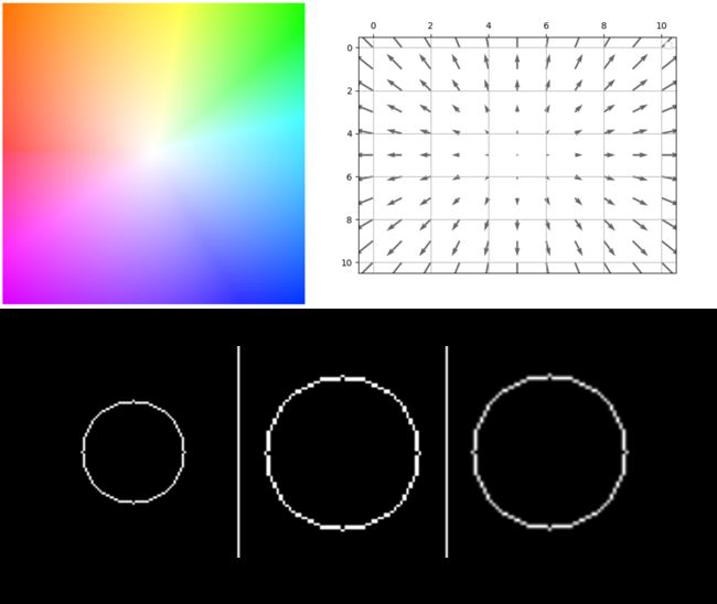
1）中心膨胀

2）向右下角偏移：

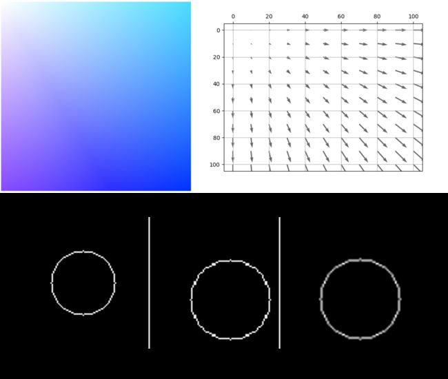
这两个例子的全部代码以公布在github上：
https://github.com/weihuang527/optical-flow