时序分析(5) -- ARMA(p,q)模型

时序分析(5)

ARMA(p,q)模型

    前两篇文章我们分别探讨了AR模型和MA模型对时序数据进行建模，这一节我们主要讨论ARMA模型。从名字中我们可以推知，ARMA模型是AR模型和MA模型的一种组合。
首先我们介绍ARMA模型的基本概念：

AutoRegression Moving Average Models - ARMA(p,q)

• AR模型是尝试捕捉和解释金融交易市场的动量和均值反转效果
• MA模型是尝试捕捉和解释在白噪声项中所观测到的振荡效果，这些震荡可以被理解为影响所观测过程的非预期事件造成的影响，例如超额收益等。

ARMA模型就是这两者的联合，它的主要缺点是忽略了在金融市场时序数据中经常可见的波动聚簇现象(Volatility Clustering)，模型公式如下：
$$y_t={\alpha }_1{y}_{t-1}+{\alpha }_2{y}_{t-2}+...+{\alpha }_p{y}_{t-p}+{\omega }_t+{\beta }_1{\omega }_{t-1}+...+{\beta }_q{\omega }_{t-q}$$
$$=\sum _{i=1}^p{\alpha }_i{y}_{t-i}+{\omega }_t+\sum _{i=1}^q{\beta }_i{\omega }_{t-i}$$

导入python包和数据

如前面系列中一样

• 模拟ARMA(2,2)过程
  下面我们以β = [0.5, −0.3，α = [0.5, −0.25]来模拟一个ARMA(2,2)过程

# Simulate an ARMA(2, 2) model with alphas=[0.5,-0.25] and betas=[0.5,-0.3]
max_lag = 30

n = int(5000) # lots of samples to help estimates
burn = int(n/10) # number of samples to discard before fit

alphas = np.array([0.5, -0.25])
betas = np.array([0.5, -0.3])
ar = np.r_[1, -alphas]
ma = np.r_[1, betas]

arma22 = smt.arma_generate_sample(ar=ar, ma=ma, nsample=n, burnin=burn)
_ = tsplot(arma22, lags=max_lag)

现在我们对此模拟数据用ARMA(2,2)进行建模

mdl = smt.ARMA(arma22, order=(2, 2)).fit(
maxlag=max_lag, method='mle', trend='nc', burnin=burn)
print(mdl.summary())

显然，ARMA模型准确的回归出了模拟数据设定的参数。

下面，我们模拟一个ARMA(3,2)过程，然后用ARMA模型来建模，搜索参数并给出赤池信息量(Akaike Information Criterion)AIC最低的p,q。

# Simulate an ARMA(3, 2) model with alphas=[0.5,-0.25,0.4] and betas=[0.5,-0.3]
max_lag = 30

n = int(5000)
burn = 2000

alphas = np.array([0.5, -0.25, 0.4])
betas = np.array([0.5, -0.3])

ar = np.r_[1, -alphas]
ma = np.r_[1, betas]

arma32 = smt.arma_generate_sample(ar=ar, ma=ma, nsample=n, burnin=burn)
_ = tsplot(arma32, lags=max_lag)
# pick best order by aic
# smallest aic value wins
best_aic = np.inf
best_order = None
best_mdl = None

rng = range(5)
for i in rng:
    for j in rng:
        try:
            tmp_mdl = smt.ARMA(arma32, order=(i, j)).fit(method='mle', trend='nc')
            tmp_aic = tmp_mdl.aic
            if tmp_aic < best_aic:
                best_aic = tmp_aic
                best_order = (i, j)
                best_mdl = tmp_mdl
         except: continue
         
print('aic: {:6.5f} | order: {}'.format(best_aic, best_order))

aic: 14266.72269 | order: (3, 2)

非常好，我们准确的找到了p,q。

print(best_mdl.summary())

我们也准确地找到了参数α, β

• 残差plot

_ = tsplot(best_mdl.resid, lags=max_lag)

残差与高斯白噪声非常拟合。

下一步，我们要尝试使用ARMA模型对四个指数数据建模。

• 国内股票收益率
  以ARMA建模， 优化目标为Max Likelihood Estimation，得到阶数为(3,2)

best_aic = np.inf
best_order = None
best_mdl = None
Y = indexs_logret['国内股票']
rng = range(5)
for i in rng:
    for j in rng:
        try:
            tmp_mdl = smt.ARMA(Y, order=(i, j)).fit(method='mle', trend='nc')
            tmp_aic = tmp_mdl.aic
            if tmp_aic < best_aic:
                best_aic = tmp_aic
                best_order = (i, j)
                best_mdl = tmp_mdl
         except: continue
print('aic: {:6.5f} | order: {}'.format(best_aic, best_order))

aic: -6601.86081 | order: (3, 2)

print(best_mdl.summary())

从拟合的模型指标上看，一阶参数都比较显著。
残差Plot

_ = tsplot(best_mdl.resid, lags=max_lag)

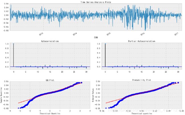
从QQ-plot上看，残差并非正态分布，所以说明模型拟合并不是非常完美。

• 香港股票收益率
  以ARMA建模
  优化目标为Max Likelihood Estimation，拟合参数为(2,2)

Y = indexs_logret['香港股票']
rng = range(5)
for i in rng:
    for j in rng:
        try:
            tmp_mdl = smt.ARMA(Y, order=(i, j)).fit(method='mle', trend='nc')
            tmp_aic = tmp_mdl.aic
            if tmp_aic < best_aic:
                best_aic = tmp_aic
                best_order = (i, j)
                best_mdl = tmp_mdl
         except: continue
print('aic: {:6.5f} | order: {}'.format(best_aic, best_order))

aic: -7640.79631 | order: (2, 2)

print(best_mdl.summary())

回归系数都比较显著

• 国内债劵收益率
  以ARMA建模
  优化目标为Max Likelihood Estimation，得到(3,1).

Y = indexs_logret['国内债券']
rng = range(5)
for i in rng:
    for j in rng:
        try:
            tmp_mdl = smt.ARMA(Y, order=(i, j)).fit(method='mle', trend='nc')
            tmp_aic = tmp_mdl.aic
            if tmp_aic < best_aic:
                best_aic = tmp_aic
                best_order = (i, j)
                best_mdl = tmp_mdl
        except: continue
print('aic: {:6.5f} | order: {}'.format(best_aic, best_order))

aic: -14105.28291 | order: (3, 1)

print(best_mdl.summary())

回归系数都比较显著

• 国内货币收益率
  以ARMA建模
  优化目标为Max Likelihood Estimation，得到(3,4).

Y = indexs_logret['国内货币']
rng = range(5)
for i in rng:
    for j in rng:
        try:
            tmp_mdl = smt.ARMA(Y, order=(i, j)).fit(method='mle', trend='nc')
            tmp_aic = tmp_mdl.aic
            if tmp_aic < best_aic:
                best_aic = tmp_aic
                best_order = (i, j)
                best_mdl = tmp_mdl
         except: continue
print('aic: {:6.5f} | order: {}'.format(best_aic, best_order))

aic: -19062.72857 | order: (3, 4)

print(best_mdl.summary())

回归系数都比较显著。

总结

    本文展示了采用Python语言为四个指数时序数据进行ARMA建模，介绍了ARMA模型的基本概念和AR、MA模型的联系，并使用ARMA模型对四指数数据进行建模。