Real-Time Rendering——Chapter 7 Advanced Shading
https://blog.csdn.net/yjr3426619/article/details/81098626 介绍brdf
https://zhuanlan.zhihu.com/p/21376124 知乎总结brdf文章
https://blog.csdn.net/NotMz/article/details/75040825
http://wiki.nuaj.net/index.php?title=BRDF#d-BRDF
https://blog.csdn.net/poem_qianmo/article/details/75943714
BRDF——bidirectional reflectance distribution function,双向反射分布函数,辐射率和辐照度的比值
辐射率是出射方向v上的辐射率;辐照度是入射方向l的辐照度。两者的比值就是BRDF,这里的双向,我的理解应该是入射方向和出射方向了。两者的比值,说明了,反射光的占入射光的百分比。不知道理解的正不正确。
Radiance 辐射率——用L表示
Irradiance 辐照度 ——光线进入,用I表示
Radiosity 或者 Radiant Existance 辐射度,辐出度,—— 光线离开,用E表示,Existance??
菲涅尔反射
在真实世界中,除了金属之外,其他物质均有不同程度的“菲涅尔效应”。视线垂直于表面时,反射较弱,而当视线非垂直于表面时,夹角越小,反射越明显。如果你看向一个圆球,那圆球中心的反射较弱,靠近边缘较强。
举个例子:如果你站在湖边,低头看脚下的水,你会发现水是透明的,反射不是特别强烈;如果你看远处的湖面,你会发现水并不是透明的,但反射非常强烈。这就是“菲涅尔效应”。
简单的讲,就是视线垂直于表面时,反射较弱,而当视线非垂直表面时,夹角越小(和水平面),反射越明显。
下面来自知乎的讲解:
https://www.zhihu.com/question/53022233
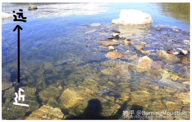
拍摄者距离河水较近,视角可以清楚的看见水下的石头,而图中较远的河水已经看不到水下的物体,水面上有较高的反射现象。

PBR并不是一项技术,它是由一系列技术的集合,并不断改进的结果。从原理到实现方案,整体来看是很复杂的,但是如果你先把每一项技术搞明白,再看清楚他们是怎么串起来的,就容易多了。把所有珍珠串起来的这根金线就是“反射率方程”。
参考:https://blog.csdn.net/Neil3D/article/details/83783638
立体角:
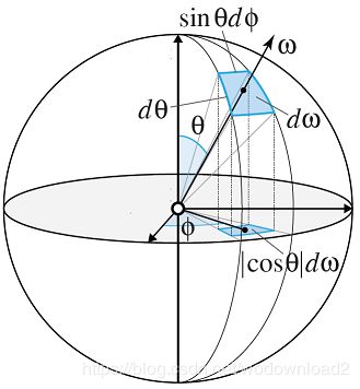
立体角并不是一个角度,而是一个面积,它是单位球面上的一个面积。
上图解释:
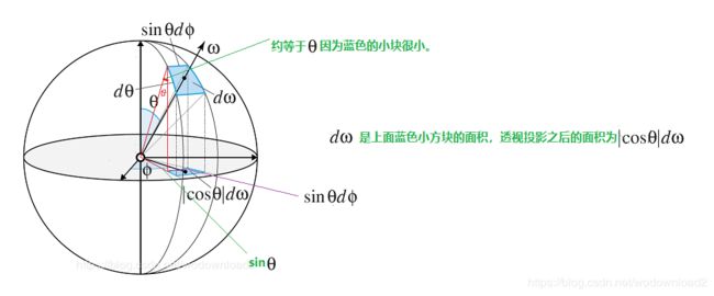
微表面
微平面理论认为,微观角度看,物体表面是由一些细小的平面组成的。微观到什么程度呢?大概可以理解为可见光波长大小的尺度。这些细小的平面,就叫做微平面。越光滑的表面,这些微平面排列的越规则,越粗糙的表面,这些微平面排列的越不规则。在图形学中,我们可以从统计学的角度使用粗糙度(roughness)这样一个估算的参数来描述这一现象。

镜面反射中Rs中的D、F、G https://blog.csdn.net/Neil3D/article/details/83783638
D:微平面分布函数(Normal distribution function)

D项,即微表面分布函数。假设表面的宏观法向量为h(就是我们常用的字母n,不知道为啥用h表示),这个函数计算得出所有微平面中法向量与n一致的微平面的比例。例如,如果有20%的微表面的法向量与n一致,则这个函数返回0.2。
unity中UnityStandardBRDF.cginc:当然unity也提供ggx模型,也同样参考这个文件:
// BlinnPhong normalized as normal distribution function (NDF)
// for use in micro-facet model: spec=D*G*F
// eq. 19 in https://dl.dropboxusercontent.com/u/55891920/papers/mm_brdf.pdf
inline half NDFBlinnPhongNormalizedTerm (half NdotH, half n)
{
    // norm = (n+2)/(2*pi)
    half normTerm = (n + 2.0) * (0.5/UNITY_PI);

    half specTerm = pow (NdotH, n);
    return specTerm * normTerm;
}
inline float GGXTerm (float NdotH, float roughness)
{
    float a2 = roughness * roughness;
    float d = (NdotH * a2 - NdotH) * NdotH + 1.0f; // 2 mad
    return UNITY_INV_PI * a2 / (d * d + 1e-7f); // This function is not intended to be running on Mobile, // therefore epsilon is smaller than what can be represented by half
}
虚幻4采用 Trowbridge-Reitz GGX 模型:

其中:
n 为表面的宏观法向量
h 入射光和观察方向的中间向量
α 为表面的粗糙度参数
G:几何遮挡因子(Geometric Occlusion Factor)
微平面理论认为,由于微平面的不规则排列,反射光有一定比率会被物体自身的微平面遮挡而衰减,这就是G项,虚幻4使用schlick模型结合smith模型计算此项,具体公式为:

F:菲涅尔项(freshnel factor)
![]()
金属以外的物体表面都会具有菲涅尔效果,虚幻4中计算菲涅尔项的公式为:
![]()
其中F0为基础反射率,是一个常数,可以通过光学测定。
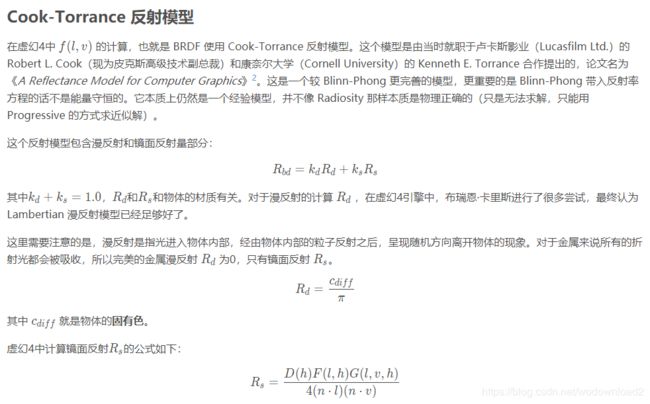
以下是来自于:http://wiki.nuaj.net/index.php?title=BRDF#d-BRDF
almost all the informations gathered here come from the reading and interpretation of the great siggraph 2012 talk about physically based rendering in movie and game production. but i have also practically read the entire documentation aout BRDFs from their first formulation by Nicodemus in 1977.
so what is a BRDF?
as i see it, it is an abstract tool that helps us to describe the macroscopic behaviour of a material when photons hit this material. it is a convenient black box, a huge multidimensional lookup table (3,4 or sometimes even 5,6 dimensions when including spatial variations) that somehow encodes the amount of photons bouning off the surface in a specific (outgoing) direction when coming from another specific (incoming) direction (and potentially, from another location).
the radiant flux of photons——or simply flux——is basically the amount of photons/energy per amount of time. and since we are considering a single CCD sensor element or a single photo-receptor in the black of the eye.
1/ we only perceive that flux in a single location, hence the “per square meter”. we need the flux flowing.
====================================================================================
The Gouraud shading model was invented in 1971 [435]. Phong’s specular highlighting equation was introduced around 1975 [1014]. The concept of applying textures to surfaces was presented a year later by Blinn and Newell [96]. As part of the standard fixed-function pipeline, these algorithms were the mainstay of graphics accelerators for years. The advent of
programmable shaders has vastly increased the available options—modern GPUs can evaluate (almost) arbitrary shading models. This moves the focus from “what is possible?” to “what are the best choices for this application?”
An understanding of the underlying physical and psychological principles pertinent to rendering is important in navigating these choices. The previous chapters presented the technologies for controlling the graphics pipeline and the basic theory behind their use. In this chapter some of the scientific underpinnings of rendering are discussed. Radiometry is presented
first, as this is the core field concerned with the physical transmission of light. Our perception of color is a purely psychological phenomenon, and is discussed in the section on colorimetry. A shading model is comprised of
two main parts: the light source and the material model. Sections on both describe the various options that are available. The final sections detail methods for the efficient implementation of shading models. The options covered in this chapter are limited by one basic assumption. Each light source is assumed to illuminate a surface location from one direction only—area, ambient, and environment lighting are not covered. Chapter 8 will describe the theory and practice necessary for the use of more general types of illumination.
7.1 radiometry
the explanation of the examle shading model in chapter 5 included a brief discussion of some concerpts from radiometry. here we will go over those concepts in more depth, and introuduce some new ones.
radiometry deals with the measurement of electromagnetic 电磁 radiation. such radiation consists of a flow of photons, which behave as either particles or waves, depending on circumstance. using the mental model of photons as particles works well for the most part. although some physical phenomena can not be modeled without accounting for the wave properties of photons, these are usually ignored by even high-quality batch rendering systems.
one wave-related property of photons that can not be disregarded is the fact that each has an associated frequency of wavelength. this is an important property, because the energy of each photon is proportional to its frequency, which affects interations between photons and matter. most importantly, it affects the interaction of photons with sensors such as the rods and cones in the human eyes. different frequencies of photons are perceived as light of different colors (or not perceived at all, if they are outside the limited range of human vision). the relationships between a photon’s wavelength λ (in meters), frequency ν (in Hertz, or cycles per second) and energy Q (in joules) are

where c is the speed of light (2.998x10^8 meters/second) and h is Planck’s constant (6.62620 × 10⁻³⁴ joule-seconds).
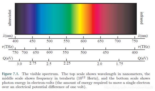
electronmagnetic radiation exists in a range of frequencies and energies, from ELF (extremely low frequency) radio waves to gamma rays. photons with wavelengths between roughly 380 to 780 nanometers are perceptible to the human eye, so only this range, the visible spectrum, is typically used for rendering. Figure 7.1 shows the colors perceived for monochromatic (singlewavelength)
light throughout the visible spectrum. Recall that photon energy is proportional to frequency: “bluer” photons are more energetic; “redder” photons are less energetic.
In this section, we will discuss the various radiometric units and their relationships. They units are summarized in Table 7.1.
![]()
in radiometry, the basic unit is energy or radiant energy Q, measured in joules (abbreviated “J”). each photon has some amount of radiant energy that, as we have seen, is proportional to its frequency. for example, at a wavelength of 550 nm, by Equation 7.1 there are 2.77x10^18 photons per joule.
the radiant flux 通量 or radiant power, Φ or P, of a light source is equal to the number of joules per second emitted (i.e., dQ/dt). the watt (W) is another term for joules per second. in principle, one can measure the radiant flux of a light source by adding up the energies of the photons it emits in a one-second time period. for example, a given light bulb may emit 100 watts of radiant flux (of which only part would be visible)——see the upper-left part of firgure 7.2.
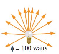
Irradiance 辐射度 (briefly discussed in chapter 5) is the density of radiant flux with respect to area (i.e., dΦ/dA).
irradiance is defined with respect to a surface, which may be an imaginary surface in space, 想象的空间, but is most often the surface of an object. in photometry, presented in the next section, the cooresponding quantity illuminance is what is measured by a light meter. as shown previously, irradiance E is used to measure light flowing into a surface and exitance M (also called radiosity or radiant exitance) is used to measure light flowing out of a surface. the general term radiant flux density is sometimes used to refer to both irradiance and exitance. chapter 5 showed how to use irradiance to measure the illumination of an ideal directional light source.
such light sources are a useful approximation for situations where the distance to the light is much larger than the extend of the rendered scene —— for example, a small pile of toys 右边的玩具 on the other side of the room from the light bulb (see the bottom part of figure 7.2). the irradiance from the light builb EL (measoured in a plane perpendicular to the light direction) is approximately constant over the scene (in this example, 0.3 watts per square meter—again, only part of this is visible radiation).

for closer light sources (or larger scenes), EL varies with distance and can not be treated as a constant. imagine concentric 同心的 spheres around the light bulb, starting at a distance much larger than the size of the bulb (see the upper-right side of figure 7.2). since the bulb is relatively small, we assume that all its light is emitted from a point at its center. we want to examine the light emitted in a particular direction (the orange arrow), so we construct a narrow cone, its axis along this direction and its apex at the center of the bulb.
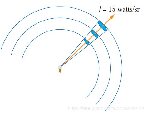
intersecting this cone with the spheres produces a sequence of patches, increasing in area proportionately to the square of their distance from the light. since the radiant flux 辐射通量 through the patches is the same, irradiance 辐射度 decreases by the same proportion:

the constant of proportionality in equation 7.2 is a value that does not change with distance:

this quantity, I, is called intensity or radiant intensity. if the distance r equals 1, then intensity is the same as irradiance——in other words, in other words, intensity is flux density with respect to area on an enclosing radius-1 sphere.
换句话说,如果在封闭的半径为1的球体内,强度=流通量密度。因为此时的r^2=1,所以I=EL
the significance of area on a radius-1 sphere can be seen from an analogy with the definition of radians弧度: an angle is a set of directions in a plane, and its size in radians is equal to the length of the arc it intersects on an enclosing radius-1 circle.
a solid angle is a three-dimensinal extension of the concept——a continuous set of directions, measured with steradians 立体角 (abbreviated “sr”), which are defined by patch area on a radius-1 sphere. solid angle is represented by the symbol ω.
from this, we can see that intensity is actually flux density with respect to solid angle (dΦ/dω), unlike irradiance, which is flux density with respect to area. intensity is measured in watts per steradian.
intensity——强度和角度有关
irradiance——辐射度和面积有关
The concept of a solid angle is sometimes difficult to grasp, so here is an analogy that may help. Solid angle has the same relationship to direction that surface area has to a surface location. Area is the size of a set of locations, and solid angle is the size of a set of directions.

most light sources do not emit the same intensity in all direction. the light bulb like this:
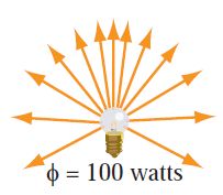
emits varying intensities of light in different directions, as can be seen from the density of arrows in the upper-left part of the figure. in the upper right, we see that the value of the light bulb’s intensity in the direction represented by the orange arrow is 15 watts per steradian.
In two dimensions, an angle of 2π radians covers the whole unit circle. Extending this to three dimensions, a solid angle of 4π steradians would cover the whole area of the unit sphere. The size of a solid angle of 1 steradian can be seen in Figure 7.3.

in the last few paragraphcs, we assumed that the light source could be treated as a point. light sources that have been approximated in this way are called point lights. just as directional lights are a useful abstraction for lights that are far away compared to the size of the scene, point lights are a useful abstraction for light sources that are far away compared to the size of the light source. itensity is useful for measuring the illumination of a point light source and how it varies with direction. as we have seen, the irradiance contribution from a point light varies inversely to the square of the distance between the point light and the illuminated surface. when is it reasonable to use this approximation? Lambert’s Photometria [716] from 1760 presents the “five-times” rule of thumb. if the distance from the light source is five times or more that of the light’s width, then the inverse square law is a reasonable approximation and so can be used.
As seen in Section 5.4, radiance L is what sensors (such as eyes or cameras) measure, so it is of prime importance for rendering. the purpose of evaluating a shading equation is to compute the radiance along a given ray (from the shaded surface point to the camera). radiance measures the illumination in a single ray of light——it is flux density with respect to both area and solid angle (see the left side of figure 7.4). the metric units of radiance are watts per square meter per steradian.
radiance 辐射率 is

where dAproj refers to dA projected to the plane perpendicular to the ray.
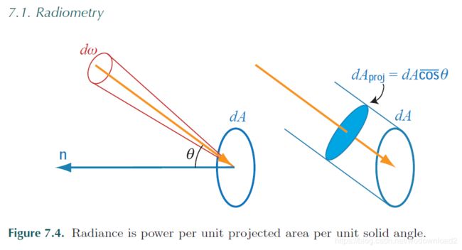
辐射率和面积还有角度有关系。一提到辐射率,就想到和面积和角度有关系,分子是辐射通量。单位面积+单位角度上的辐射量。
那么我们自然会想到,如果是分别和面积或者角度有关的辐射量,又叫啥呢?辐射率用L表示。
比如辐射量和单位面积上的比值,叫做辐照度(光线射到物体表面);或者叫做辐出度,关系在表面上反射出来的量,辐照度后者辐出度用E表示。
再比如辐射量和单位角度的比值,叫做辐射强度。单位角度是立体角。辐射强度用I表示
the relationship between dA and dAproj can be seen in the right side of figure 7.4, where we see that the projection depends on the cosine of θ, the angle between the ray and the surface normal n:

Note that Equation 7.5 uses the cos(上面一横杠) symbol (defined on page 8), which represents a cosine clamped to zero. Negative cosine values occur when the projected direction is behind the surface, in which case the projected area is 0.
A density with respect to two quantities simultaneously is difficult to visualize. It helps to think of radiance in relation to irradiance or intensity:

where Eproj refers to irradiance measured in the plane perpendicular to the ray. Figure 7.5 illustrates these relationships.
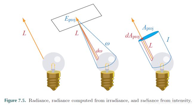
The ray exiting the light bulb in the left side of Figure 7.5 has radiance L. In the middle of the figure we see the relationship between L and the irradiance Eproj from the light bulb (measured at a surface perpendicular to the ray). This irradiance is the flux density per area at a surface point— it represents photons hitting that point from all parts of the light bulb, covering a range of directions represented by the solid angle ω. As seen in the right side of Equation 7.6, the radiance L is the density of E per solid angle. This is computed for a given direction by looking at only the irradiance contributed by photons arriving from a small solid angle dω around that direction and dividing that irradiance by dω.
On the right side of Figure 7.5 we arrive at radiance “the other way,” starting with intensity I. Intensity represents all photons from the light
bulb going in a certain direction, from all parts of the light bulb, covering a projected area Aproj. As seen in the left side of Equation 7.6, the radiance L is the density of I per area. This is computed for a given point by looking at only the intensity contributed by photons passing through a small area dAproj around the given direction and dividing that irradiance by dAproj.
7.5 BRDF theory
section 5.5 described a shading equation for simulating interation of light with a surface. this equation is just one of many possible shading equations that can be used. in this section we will explain the theory behind such equations, go over some of the more interesting possibilites, and finally discuss implementation issues.
7.5.1 The BRDF
When shading a surface, the outgoing radiance in a given direction is computed, given quantities and directions of incoming light. In radiometry, the function that is used to describe how a surface reflects light is called the bidirectional reflectance distribution function (BRDF) [932].
As its name implies, it is a function that describes how light is reflected from a surface given two directions—the incoming light direction l and outgoing view direction v.
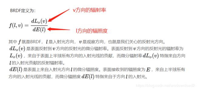
The precise definition of the BRDF is the ratio between differential outgoing radiance 辐射率 and differential irradiance 辐射通量密度:

to understand what this means, imagine that a surface is illuminated by light incoming from a tiny solid angle (set of directions) around l. This illumination is measured at the surface as irradiance dE. The surface then reflects this light in various directions. In any given outgoing direction v, the radiance dLo is proportional to the irradiance dE. The ratio between the two, which depends on l and v, is the BRDF. The value of the BRDF depends also on wavelength, so for rendering purposes it is represented as an RGB vector.
我们的分母是辐照度,表示光线到达表面的通量(单位面积),只和面积有关系。
分子是光线离开表面的,辐射率。和面积和单位立体角有关系。
The discussion in this chapter is restricted to shading with non-area light sources such as point or directional lights. In this case, the BRDF
definition can be expressed in a non-differential form:

where EL is the irradiance 辐照度 of a light source measured in a plane perpendicular to the light direction vector l, and Lo(v) is the resulting outgoing radiance in the direction of the view vector v. The clamped cosine of the angle θi between l and the surface normal n converts EL to irradiance measured at the surface. It is now straightforward to see how the BRDF fits into a general shading equation with n non-area lights:

where k is the index for each light.
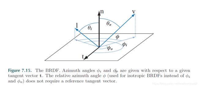
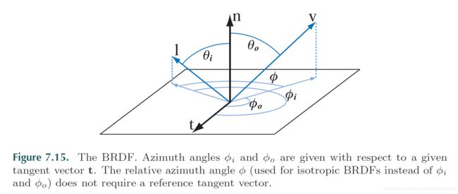
The ⊗ symbol (piecewise vector multiply) is used, since both the BRDF and irradiance are RGB vectors. Since the incoming and outgoing directions each have two degrees of freedom (a common parameterization is to use two angles: elevation θ relative to the surface normal and rotation φ about the normal), the BRDF is a function of four scalar variables in the general case. Isotropic BRDFS are an important special case. Such BRDFs remain the same when the incoming and outgoing direction are rotated around the surface normal (keeping the same relative angles between them). Isotropic BRDFs are functions of three scalar variables. Figure 7.15 shows the variables used in both cases.
The BRDF is defined as radiance (power/(area × solid angle)) divided by irradiance (power/area), so its units are inverse solid angle, or
steradians−1. Intuitively, the BRDF value is the relative amount of energy reflected in the outgoing direction, given the incoming direction.
Figure 7.16. Light interacting with a surface. On the left, we see the subsurface interactions causing light to be re-emitted away from the entry point. The red and green circles represent the region covered by a pixel at two different scales of observation. On the right, all subsurface scattered light is shown emitting from the entry point—the details of what happens under the surface are ignored.
The BRDF abstracts how light interacts with an object. Section 5.3 discussed the various phenomena that occur: Some light is scattered into the surface (refraction or transmission), and some light is scattered away (reflection). In addition, the light transmitted into the object may undergo absorption and additional scattering, eventually causing some of it to exit the surface—a phenomena called subsurface scattering. The left side of Figure 7.16 shows these various types of light-matter interactions.
Figure 7.16 also contains two colored circles that show the areas covered by a pixel in two cases. The red circle represents a case where the area covered by a pixel is small compared to the distance between the entry and exit locations of the subsurface scattered light. In this case, a BRDF cannot be used to describe the subsurface scattering; instead a more general equation must be used. This equation is the bidirectional surface scattering reflectance distribution function (BSSRDF) [932]. The general BSSRDF encompasses large-scale subsurface scattering by adding incoming and outgoing locations as inputs to the function. The BSSRDF describes the relative amount of light that travels along the incoming direction, then from one point to the other of the surface, then along the outgoing direction. Techniques for rendering objects that exhibit large-scale subsurface scattering will be discussed in Section 9.7.
The green circle in the left side of Figure 7.16 represents a case where each pixel covers a larger area (perhaps the camera is farther away). In this case, the pixel coverage is large, compared to the scale at which the subsurface scattering occurs. At this scale reflection, refraction and subsurface scattering can be approximated as happening at a single point, as seen in the right side of the figure.
This approximation enables modeling all the light interaction—including subsurface scattering—with a BRDF. Whether a BRDF can be used depends both on the surface material (for example, subsurface scattering occurs over larger distances in wax than in marble) and on the scale of observation (for example, rendering a close-up of the face of a marble statue versus a long shot of the entire statue). The original derivation of the BRDF as an approximation of the BSSRDF [932] defined the BRDF as a property of uniform surfaces, where the BRDF was assumed to be the same over the surface. Objects in the real world (and in rendered scenes) rarely have uniform material properties over their surface; even an object that is composed of a single material (e.g., a solid gold statue) will have variations in surface roughness, corroded and dirty spots, etc., which will cause its visual properties to change from one surface point to the next. A function
that captures BRDF variation based on spatial location is called a spatially varying BRDF (SVBRDF) or spatial BRDF (SBRDF). Even the general BSSRDF, as complex as it is, still omits variables that can be important in the physical world, such as the polarization of the light [1089]. Also, transmission of light through a surface is not handled, only reflection [409]. To handle transmission, two BRDFs and two BTDFs (“T” for “transmittance”) are defined for the surface, one for each side, and so make up the BSDF (“S” for “scattering”). In practice, these more complex functions are rarely needed, and a BRDF or SVBRDF is sufficient to model most surface behavior.
BRDF Characteristics
The laws of physics impose two constraints on any BRDF. The first constraint is Helmholtz reciprocity Helmholtz reciprocity 赫尔姆霍兹互惠, which means that the input and output angles can be switched and the function value will be the same:

In practice, BRDFs used in rendering often violate 违反 Helmholtz reciprocity without noticeable artifacts. However, it is a useful tool to use
when determining if a BRDF is physically plausible 有道理的. The second constraint is conservation of energy 能量守恒—the outgoing energy cannot be greater than the incoming energy (not counting glowing surfaces that emit light, which are handled as a special case 这里不考虑自发光的情况).
Certain offline rendering algorithms (e.g., some kinds of ray tracing) require energy conservation. For real-time rendering, strict energy conservation is not necessary, but approximate energy conservation is desirable. A surface rendered with a BRDF that grossly violates energy conservation might look much too bright, decreasing realism.
对于离线渲染的算法,比如光线跟踪,严格遵守能量守恒;但是对于实时渲染没有必要严格遵守,但是近似的遵守能量守恒还是必要,如果
The directional-hemispherical reflectance R(l) is a function related to the BRDF. It can be used to measure to what degree a BRDF is energyconserving. Despite its somewhat daunting name, the directional-hemispherical reflectance is a simple concept. It measures the amount of light coming from a given direction that is reflected at all, regardless of outgoing direction. Essentially, it measures energy loss for a given incoming direction. The input to this function is the incoming direction vector l, and its definition is the ratio between differential exitance and differential irradiance, as shown in Equation 7.23:
辐出度和辐照度的比值

Since the discussion is restricted to non-area light sources in this chapter, a simpler, non-differential definition can be used:

where EL is the irradiance of a light source measured in a plane perpendicular to the light direction vector l, and M is the resulting exitance (recall that exitance is the same as irradiance, but for outgoing light).
M表示的是辐出度。
the value of the directional-hemispherical reflectance R(l) must always be between 0 and 1 (as a result of energy conservation). a reflectance value of 0 represents a case where all the incoming light is absorbed or otherwise lost. if all of the light is reflected, the reflectane will be 1. in most cases it will be somewhere between these two values. Like the BRDF, the values of R(l) vary with wavelength, so it is represented as an RGB vector for rendering purposes. Since each component (R, G and B) is restricted to lie between 0 and 1, a value of R(l) can be thought of as a regular color. note that this restriction does not apply to the values of the brdf! As a distribution function, the BRDF can have arbitrarily high values in certain directions (such as the center of a highlight) if the distribution it describes
is highly non-uniform.
The directional-hemispherical reflectance is closely related to the BRDF. The relationship between them is presented in Equation 7.25:

The Ω subscript on the integral sign means that the integral is performed over the hemisphere above the surface (centered on the surface normal n).
7.5.2 surface and body reflectance
to choose brdfs for rendering, it is useful to understand the behaviour of light when interacting with real-world objects. to have a clear mental model of this interaction, it is important to differentiate between the pheomena that occur at the object’s infinitely thin surface, and those occuring under the surface, in the object’s interior (this distinction was briefly discussed in Section 5.3). when using brdf representations, surface phenomena are simulated as surface reflectance, and interior phenomean are modeld as body reflectance (the term volume reflectance is also sometimes used). the surface is an optical discontinuity 光学不连续的, and as such scatters light (causes it to change direction) but does not abosorb any; all incoming light is either reflected or transmitted. The object’s interior contains matter,
which may absorb some of the light. It may also contain additional optical discontinuities that will further scatter the light (subsurface scattering).
this is why it is meaningful to talk about surface transmission and refraction even in highly absorptive materials. Absorption occurs under the surface, perhaps very close to it, but never at the surface itself. Surface reflectance is typically modeled with specular BRDF terms—body reflectance is modeled with diffuse terms.
7.5.3 fresnel reflectance
an object’s surface is an interface between two different substances: air and the object’s substance. the interaction of light with a planar interface between two substances follows the fresnel equations developed by Augustin-Jean Fresnel (pronounced freh-nel) in the 19th century. in theory, the fresnel equations require a perfect plane, which of course is not possible in a real surface. even if the surface is perfectly flat at the atomic level (very difficult to achieve!) the atoms themselves form “bumps”. in practice, any irregularities much smaller than the smallest light wavelength (about 400 nanometers in the case of visible light) have no effect on the light, so a surface that possesses only such irregularities 不规则 can be considered a perfect plane for optical purposes. In Section 7.5.6 we will see how to
apply Fresnel reflectance to rougher surfaces. Note that Fresnel reflectance is strictly a surface reflectance phenomenon, independent of any body reflectance phenomena such as absorption.
Recall that optical discontinuities cause light to scatter, or change direction. 由于表面的不光滑,导致光学改变反向,向四周反射。an optically planar interface between two substances is a special case, which scatters each ray of incoming light into exactly two directions:
the ideal reflection direction and the ideal refraction direction (see the left side of Figure 7.18).

note that the ideal reflection direction (indicated by the vector ri) forms the same angle (θi) with the surface normal n as the incoming direction l.The ideal refraction or transmission vector t forms a different angle (θt) with the negated surface normal −n. All these vectors are in the same plane. The amount of light reflected is described by the Fresnel reflectance RF , which depends on the incoming angle θi. due to conservation of energy, any light not reflected is transmitted, so the proportion of transmitted flux to incoming flux is 1 − RF . The proportion of transmitted-to-incident radiance, however, is different. Due to differences in projected area and solid angle between the incident and transmitted rays, the relationship between the incident and transmitted radiance is

The reflection vector ri can be computed from n and l:
The right side of Figure 7.18 shows a geometrical construction that explains Equation 7.30.
Both the Fresnel reflectance RF and the transmission angle θt depend not only on the incoming angle θi, but also on an optical property of the two substances called the refractive index or index of refraction. The symbol n is commonly used to denote refractive index. In this case n1 is the refractive index of the substance “above” the interface (where the light is initially propagating) and n2 is the refractive index of the substance “below” the interface (where the refracted light propagates). The dependence of θt on θi, n1, and n2 obeys a simple equation, known as Snell’s Law:
The vector t is used in global refraction effects, which are outside the scope of this chapter; the use of Snell’s Law to efficiently compute t will be shown in Section 9.5. Snell’s Law combined with Equation 7.29 yields a different form for transmitted radiance:
The Fresnel equations describe the dependence of RF on θi, n1, and n2. Rather than present the equations themselves (which are quite complicated), we will describe their important characteristics.
External Reflection
External reflection is the case where light reflects from an object’s external surface; in other words, light is in transition from air to the object’s substance (the opposite transition, from object to air, is called internal reflection and is discussed later).
For a given substance, the Fresnel equations can be interpreted as defining a reflectance function RF (θi), dependent only on incoming light angle. In principle, the value of RF (θi) varies continuously over the visible spectrum. For rendering purposes its value is treated as an RGB vector. The function RF (θi) has the following characteristics:
- When θi = 0◦ (light perpendicular to the surface, or l = n) RF (θi) has a value that is a property of the substance. This value, RF (0◦), can be thought of as the characteristic specular color of the substance. The case when θi = 0◦ is sometimes called normal incidence,
- As θi increases (the surface is viewed at increasingly glancing angles), the value of RF (θi) will tend to increase, reaching a value of 1 for all frequencies (white) at θi = 90◦.
Figure 7.19 shows RF (θi) curves for external reflection from a variety of substances. The curves are highly nonlinear—they barely change until θi = 60◦ or so, and then quickly go to 1. The increase from RF (0◦) to 1 is mostly monotonic, though some of the substances (most notably aluminum) do show a slight dip just before going to white.
This increase in reflectance at glancing angles is sometimes called the Fresnel effect in rendering. You can see the Fresnel effect for yourself with a short experiment. Take a plastic CD case and sit in front of a bright area like a computer monitor. First hold the CD case close to your chest, look down at it, and angle it slightly so that it reflects the monitor. There should be a relatively weak reflection of the monitor on the plastic, and the CD or cover image should be clearly visible under it. This is because the characteristic, normal-incidence reflectance of plastic is quite low. Now raise the CD case up so that it is roughly between your eyes and the monitor, and again angle it to reflect the monitor. Now the reflection of the monitor should be much stronger, obscuring whatever is under the plastic.
Besides their complexity, the Fresnel equations have other properties that makes their direct use in rendering difficult. They require (possibly complex) refractive index values sampled over the visible spectrum. The equations are evaluated for all the sampled frequencies and converted into RGB values using the methods detailed in Section 7.3.

The curves in Figure 7.19 suggest a simpler approach based on the
characteristic specular color RF (0◦). Schlick [1128] gives an approximation
of Fresnel reflectance that is fairly accurate for most substances:
![]()
7.5.4 local subsurface scattering
metals and semiconductors quickly absorb any transmitted light, so body reflectance is not present, and surface reflectance is sufficient to describe the interaction of light with the object. for insulators绝缘体, rendering needs to take account of body reflectance as well.
if the insulator is homogenous ———with few internal discontinuties to scatter light——then it is transparent. common examples are glass, gemstones, crystals, and clear liquids such as water, oil, and wine. such substances can partically absorb light traveling though them, but do not change its direction. Transmitted light continues on a straight line through such objects until it undergoes internal reflection and transmission out of the object. techniques for rendering such substances are discussed in sections 5.7, 9.4, 9.5 and 10.16.
most insulators (including common substances such as wood, stone, snow, earth, skin, and opaque plastic——any opaque non-metal) are heterogeneous异构的——they contain numberous discontinuities, such as air bubbles, foreign particles, density variations, and structural changes. these will cause light to scatter inside the substance. as the light travels through the substance, it may be partially or completely absorbed. eventually, any light not absorbed is re-emitted from the surface. to model the reflectance with a BRDF, it is necessary to assume that the light is re-emitted from the same point at which it entered. we will call this case local subsurface scattering. methods for rendering in cases where this assumption can not be made (global subsurface scattering) are discussed in section 9.7.
the scattering albedo ρ of a heterogeneous insulator is the ratio between the energy of the light that escapes a surface compared to the energy of the light entering into the interior of the material. the value of ρ is between 0 (all light is absorbed) and 1 (no light is absorbed) and can depend on wavelength, so ρ is modeled as an RGB vector for rendering. one way of thinking about scattering albedo is as the result of a “race” between absorption and scattering
未完待续
7.5.5 microgeometry
the previous sections discussed material properties relating to the composition or internal structure of the object, with the surface assumed to be optically flat. most real surfaces exhibit some roughness or structure that affects how light reflects from them. surface detail modeled by a brdf is microscale——smaller than the visible scale or, in other words, smaller than a single pixel. larger details are typically modeled with textures or geometry, not with BRDFs. as we dicussed in section 5.3, whether surface structures are considered to be microscale depends on the scale of observation as much as on the size of the structures themselves.
since such microgeometry is too small to be seen directly, its effect is expressed statistically in the way light scatters from the surface. the microscale structures or irregularities are assumed to be significantly larger than visible light wavelengths (approximately 400 to 800 nanometers). This is because structures have no effect on the light if they are much smaller than visible light wavelengths. If the size is on the same order as the wavelength, various wave optics effects come into play [44, 515, 1213, 1345, 1346]. Surface detail on this scale is both difficult to model and relatively rare in rendered scenes, so it will not be further discussed here.
the most important visual effect of the microgeomery is due to the fact that many surface normals are present at each visible surface point, 一个点有多个法线? rather than a single macroscopic surface normal. since the reflected light direction is dependent on the surface normal (recall equation 7.30)

this causes every incoming light ray to be reflected into many directions; see figure 7.23.
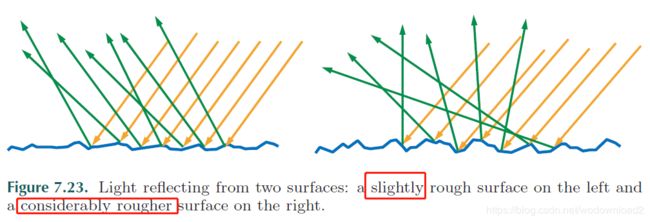
since we cannot see that the microgeometry surface normals and their directions are somewhat random, it makes sense to model them statistically, as a distribution. 分布 for most surfaces, the distribution of microgeometry surface normals is a continuous distribution with a strong peak at macroscopic surface normal. the “tightness” of this distribution is determined by surface smoothness. on the right side of figure 7.23, we see light reflecting from a surface that is rougher (and thus has its microgeometry normals clustered less tightly around the overall surface normal) 法线不紧凑?? than the surface on the left side of the figure. note that the wider distribution of normals causes the reflected light to “spread” in a wider range of directions.

the visible effect of increasing microscale roughness is greater blurring of reflected environmental detail. in the case of small, bright light sources, this blurring results in broader and dimmer 暗 specular hightlights (highlights from rougher surfaces are dimmer because the light energy is spread into a wider cone of directions). this can be seen in the photographs in figure 5.8 on page 106. 243
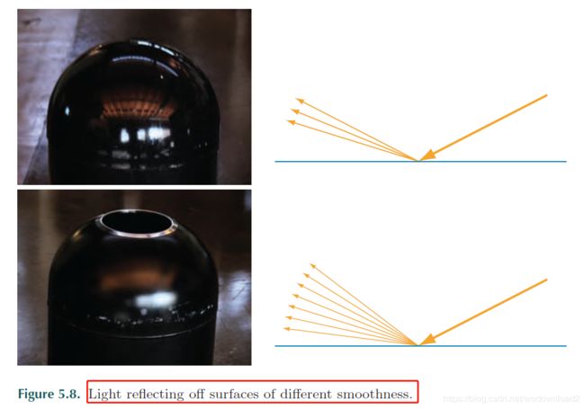
figure 7.24 shows how visible reflectance results from the aggregate reflections of the individual microscale surface details. 叠加之后的反射效果。the series of images shows a curved surface lit by a single light, with bumps that steadily decease in scale until in the last image the bumps are all smaller than a single pixel. it can be seen that statistical patterns in the many small highlights eventually become details in the shape of the resulting aggregate highlight. for example, the relative sparsity 稀疏 of individual bump highlights in the periphery 外围 becomes the relative darkness of the aggregate hightlight away from its center.
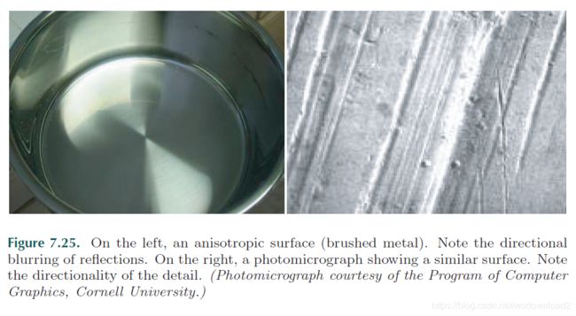
for most surfaces, the distribution of the microscale surface normals is isotropic各向同性——rotationally symmetrical 严格对称的, or lacking any inherent directionality. however, some surfaces have miscroscale structure that is anisotropic. this results in anisotropic surface normal distributions, and directional blurring of reflections and highlihgts (see figure 7.25).
some surfaces have highly structured microgeometry, resulting in interesting microscale normal distributions and surface appearance. fabrics are a commonly encountered example——the unique appearance of velvet and satin is due to the structure of their microgeometry.
although multiple surface normals are the primary effect of microgeometry on reflectance, other effects can also be important. shadowing refers to occlusion of the light source by microscale surface detail, as shown on the left side of figure 7.26. masking ((visibility occlusion of microscale surface detail) is shown in the center of the figure.

if there is a correlation between the microgeometry height and the surface normal, then shadowing and masking cna effectively change the normal distribution. for example, imagine a surface where the raised parts have been smoothed by weathering or other processes, and the lower parts remain rough. at glancing angles, the lower parts of the surface will tend to be shadowed or masked, resulting in an effectively smoother surface. see figure 7.27.
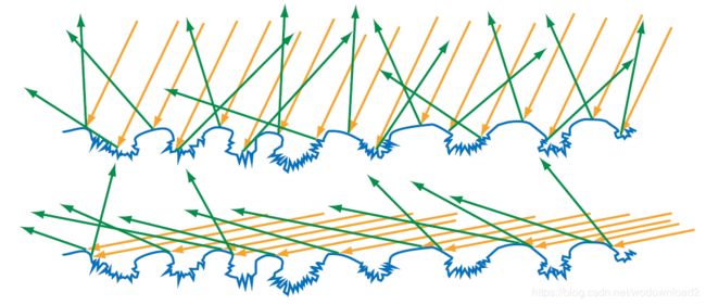
figure 7.27. microgeometry with a strong correlation between height and surface normal (raised areas are smooth, lower areas are rough) 微几何领域,法线和高度有这密切的联系,凸起的地方更光滑,低凹的地方则粗糙。in the top image, the surface is illuminated from an angle close to the macroscropic 宏观的 surface normal. 入射的光线和宏观的法线很贴近。at this angle, the rough pits are accessible to many of the incoming light rays, and many of them are scattered in different directions. 在这样的角度下照射,低凹处的粗糙部分,会接收到很多的光线。入射的光线向四面八方进行漫反射。in the bottom image, the surface is illuminated from a glaning angle. 上图中处于下方的图,是以一个很接近平面的斜视角进行照射. shadowing blocks most of the pits, so few light rays hit them, and most rays are reflected from the smooth parts of the surface. 凹处的部分处于阴影之中,接收很少一部分的光线,更多的光线是在高处的那些平滑的地方进行反射。in this case, the apparent roughness depends strongly on the angle of illumination. 这种情况下,很显然粗糙程度和照亮的角度有关。
In addition, the effective size of the surface irregularities is reduced as the incoming angle θi increases. At extremely glancing angles, this can decrease the effective size of the irregularities to be shorter than the light’s wavelength, making the surface optically smooth.
正如上图中展示的,当入射角度越大的时候,表面的粗糙度反而减少了,当达到一个极端的角度时,表面的不规则形状将减少到比光波的波长还小,这样表面就接近于理想的光滑程度了。
These two effects combine with the Fresnel effect to make surfaces appear highly reflective and mirror-like as the viewing and lighting angles approach 90◦ [44, 1345, 1346]. Confirm this for yourself: Put a sheet of non-shiny paper nearly edge on to your eye, looking off it toward a computer screen. Hold a pen with a dark surface along the far edge, so that it points out from the paper. At a very shallow angle you will see a reflection of the pen in the paper. The angle has to be extremely close to 90◦ to see the effect.
这个实验怎么做?不太明白
Light that was occluded by microscale surface detail does not disappear— it is reflected, possibly onto other microgeometry. Light may undergo multiple bounces in this way before it reaches the eye. Such interreflections are shown on the right side of Figure 7.26.
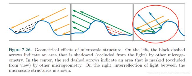
Since the light is being attenuated by the Fresnel reflectance at each bounce, interreflections tend not to be noticeable in insulators 绝缘体. In metals, multiple-bounce reflection is the source of any visible diffuse reflection (since metals lack subsurface scattering).
Note that multiple-bounce reflections from colored metals are more deeply colored than the primary reflection, since they are the result of light interacting with the surface multiple times.
由菲涅尔反射得到,每次的反射光的能量都会衰减,在绝缘体中这种多次的反射可能不太明显,但是在金属材质中,多次的反射是漫反射的主要来源,这是因为金属更多发生的是反射而不会被吸收。而且对于有色金属来说,多次反射比一次反射,颜色要更加明显,因为光在多次与表面交互之后色彩更加明显。
So far we have discussed the effects of microgeometry on specular, or surface reflectance. In certain cases, microscale surface detail can affect body reflectance, as well. If the scale of the microgeometry is large relative to the scale of subsurface scattering (the distances between the entry and exit points of subsurface-scattered light), then shadowing and masking can cause a retro-reflection effect, where light is preferentially reflected back toward the incoming direction. This is because shadowing and masking will occlude lit areas when the viewing and lighting directions differ greatly (see Figure 7.28).

figure 7.28. retro-reflection due to microscale roughness. both sides show a rough surface with low fresnel reflectance and high scattering albedo (so body reflectance is visually important). on the left, the viewing and lighting directions are similar. the parts of the microgeometry that are brightly lit are also the ones that are highly visible, leading to a bright appearance. one the right, the viewing and lighting directions differ greatly. in this case, the brightly lit areas are occluded from view and the visible areas are shadowed. this leads to a darker appearance.
观察上面的两个图,左边的图,入射光和视角方向基本一致,所以该照亮的部分,也照亮了。而右边的,入射光的方向和观察的方向相聚很远,本该照亮的部分,由于被凸起的部分遮挡,所以显得很暗。
This retro-reflection effect 逆反射效应 will tend to give rough surfaces a flat appearance (this is why the moon appears as a flat disc and does not look like a Lambert-shaded sphere). Figure 7.29 shows photographs of two objects exhibiting this behavior.
7.5.6 microfacet theory
many BRDF models are based on a mathematical analysis of the effects of microgeometry on reflectance called microfacet theory. microfacet theory was developed in its moden form by torrance and sparrow and was introduced to computer graphics in 1977 by blinn and again in 1981 by cook and torrance. this theory is based on the modeling of microgeometry as a collection of microfacets. each microfacet is a tiny, flat fresnel mirror on the surface. in microfacet theory, a surface is characterized by the distribution of the microfacet surface normals. this distribution is defined by the surface’s normal distribution function, or NDF.
这里有的网址将其翻译为正太分布函数,真的太搞笑了。应该译为法线分布函数。
we will use p() to refer to the NDF in equations. the NDF is defined as the probability distribution function of the microfacet surface normals. the probability that the surface normal of a given microfacet lies within an infinitesimal solid angle dw surrouding a candidate direction vector nu is equal to p(nu)dw. for a function to be a valid NDF, it needs to be normalized so that it integrates to 1 over the sphere, since the possibility of a microfacet normal pointing somewhere is 1. intuitively, the NDF is similar to a histogram of the microfacet normals; it has high values in directions where the microfacet normals are more likely to be pointing. NDF是类似于微表面的法线的直方图,在和宏观法线重合的时候,直方图达到了最高点。
most surfaces have NDFs that show a strong peak at the macroscopic宏观的 surface normal n. in other words, the microfacets are likely to be oriented similarly to the overall macroscopic surface. 微表面的法线和宏观的法线方向近似。section 7.6 will discuss a few different NDF models used in rendering.

figure 7.30. surface composed of microfacets. only the red microfacets, which have their surface normal aligned with the half vector h, participate in the reflection of light from the incoming light vector l to the view vector v.
7.6 BRDF models
in most applications BRDFs are represented analytically, as mathematical equations. Many such models have appeared in the computer graphics literature, and several good surveys are available [44, 926, 1129, 1170, 1345, 1346]. BRDF models fall into two broad groups: those based on physical theory [41, 97, 192, 193, 515, 640, 973, 1027, 1213] and those that are designed to empirically fit a class of surface types [42, 43, 1014, 1326]. 两派:物理的+经验模型
since the emprical BRDF models tend to be simpler, they are more commonly used in real-time rendering. the first such model used in rendering was the Lambertian or constant BRDF. phong introduced the first specular model to computer graphics in 1975 [1014]. this model is still in common use; however, it has several drawbacks that merit discussion 有几个缺点值得讨论. The form in which the Phong lighting model has historically been used (shown with a single light source for simplicity) is 只考虑一盏灯

the use of BL rather than EL is due to the fact that this form of the shading equation does not use physical illumination quantities, but rather uses ad hoc “brighness” values assigned to light sources. Recall from Section 7.5.4 that effectively BL = EL/π. Using this and Equation 7.21, we can transform Equation 7.44 into a BRDF:


Comparing this to Equation 7.36 on page 240 shows that Cdiff is equal to the directional-hemispherical reflectance of the diffuse term. This is fortunate—reflectance values make very good BRDF parameters. As a reflectance value,作为反射率的值,Cdiff在0和1之间。 Cdiff is restricted to values between 0 and 1, so it can be selected with color-picker interfaces, stored using standard texture formats, etc. The fact that Cdiff has a clear physical interpretation can also be used to help select appropriate values for it.
It would be useful to ensure that Cspec is a reflectance value, as well. To do this, we need to look at the directional-hemispherical 方向半球reflectance Rspec of the specular term. However, it turns out that for Equation 7.45, Rspec is unbounded, Rspec是没有边界, increasing to infinity as θi goes to 90◦ [769]. This is unfortunate—it means that the BRDF is much too bright at glancing angles. The cause of the problem is the division by cosθi. Removing this division also allows us to remove the conditional term, resulting in a simpler BRDF:
当θi=90度的时候,cosθi=0,除以这个值,得到无穷大。

This version of the Phong BRDF is more physically plausible in several ways—its reflectance does not go to infinity, it is reciprocal, and it lacks the abrupt cutoff when θi = 90◦. An example of an artifact caused by this cutoff can be seen in Figure 7.35.
phong 的BRDF有有好处也有坏处,就是舍去了θi=90的情况,导致下面的人造结果:

Figure 7.35. The cutoff in Equation 7.45 when θi = 90◦ can cause artifacts, as seen by the unnatural line towards the bottom right of the figure.
The directional-hemispherical reflectance of the specular term in Equation 7.46 can now be calculated. It turns out that when θi = 0, it reaches a maximum value of 2Cspec/(m + 2). If we divide the specular term by 2/(m + 2), then Cspec will be equal to the maximum directional hemispherical reflectance [586]:
当θi = 0,反射系数达到最大为:2Cspec/(m + 2)
我把反射系数除以2/(m + 2),得到下面的式子:这里不太懂了。。。。
其实就是normalized,当θi = 0时,得到最大的反射系数,那么除以这个系数2/(m + 2),就归一化到了0到1之间。

This process of multiplying a BRDF term by a value to ensure that parameters such as Cspec are equivalent to reflectance values is called BDRF normalization. The value by which the term is divided is called a normalization factor, and the resulting BRDF is referred to as a normalized BRDF. 规格化的BRDF
Normalized BRDFs have many advantages over non-normalized ones. We have already discussed the benefits of color parameters being closely related to reflectance values. In this case Cspec is equal to the maximum value of the directional-hemispherical reflectance of the specular term, which in turn is closely related to the Fresnel reflectance at normal incidence RF (0◦). Since Equation 7.47 does not account for the Fresnel effect, using cspec = RF (0◦) will probably be too dark. Using a value for cspec that is partway between white and RF (0◦) may work better. If energy conservation is desired (it can sometimes be a useful guideline to help ensure realism), this can be guaranteed by ensuring that cdiff + cspec ≤ 1.
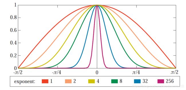
Another important effect of normalization is that now the m parameter is independent of reflectance and only controls surface roughness. m是用来控制粗糙度的?是的,回忆之前计算镜面反射的时候,有一个pwer系数,系数越高,高光越集中,越集中代表材质越光滑,所以这里的m用来控制粗糙度。
figure 7.36. graph of unnormalized cosine power term versus angle for various exponents. increasing the exponent pulls the curve in, making for a tighter highlight. however, the height of the curve remains unchanged. this causes the total specularly reflected energy to decrease.
the non-normalized version of the BRDF, chaning m changed both the amount and distribution of outgoing light. to understand why, to understand why, see figure 7.36. with higher exponents, the width of the curve (and thus the size of the rendered highlight) decreases; however the peak of the curve (the brightness at the highlight center) remains the same. the overall energy in the highlight decreases, since it is related to the intergral under this curve.
this behaviour was necessary when graphics hardware could not handle values outside the 0 to 1 range, but, it is avoidable today and is undesirable. with non-normalized BRDFs, adjusting the surface roughness changes the reflectance was a side effect. this is bad because the reflectance defines the perceived specular color. this color defines the “look” of gold, copper, glass, etc. independent of surface roughness. for example, with a normalized BRDF an artist can set the overall specular color of a gold statue 雕像 to the appropriate value (see table 7.4) and then paint a roughness map with detail to show where the statue is smooth and where it is rough. the rough and smooth areas with both look like gold. if a non-normalized BRDF is used, then to get the correct gold appearance, the artist would need to use a second texture controlling the specular color and painstakingly 煞费苦心地 paint values into it that would compensate for the roughness values. worse still, depending on the surface roughness, these values could be very small or very large, making it difficult or impossible to store them in a texture.
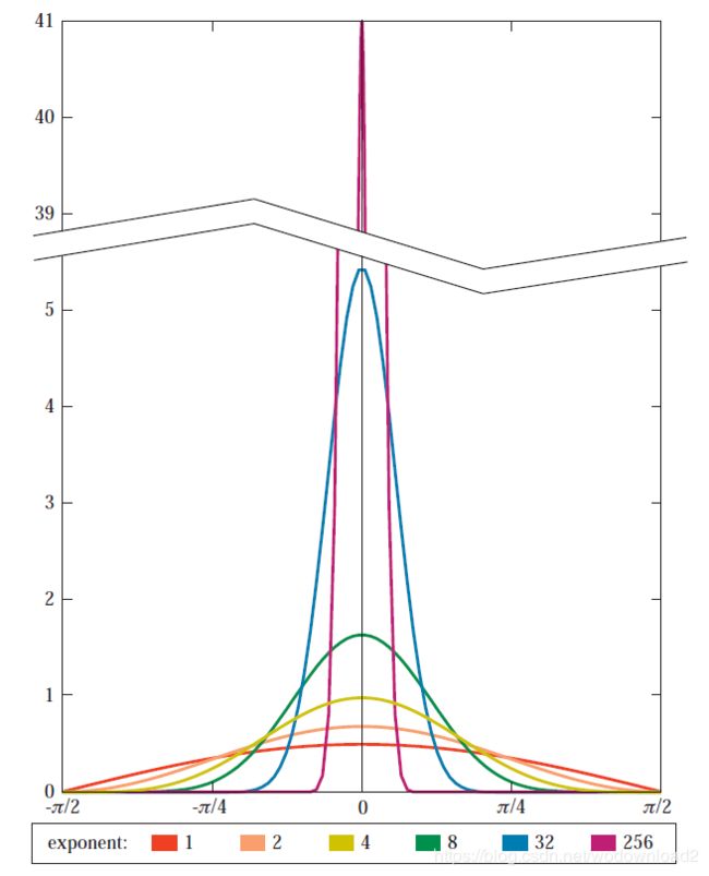
figure 7.37. graph of normalized cosine power term versus angle for various exponents. increasing the exponent not only makes the curve narrower, but also higher. this increase in height compensates for the decrease in width, keeping the total reflected energy constant.
compare this graph to figure 7.37, which shows normalized curves. when the exponent increases (corresponding to a smoother surface), the size of the highlight decreases, but its brightness increases, keeping the total reflectance constant. recall that although reflectance values such as R are limited to the 0 to 1 range, BRDF values can (and often do) exceed 1, especially in the case of smooth surfaces.
figure 7.38 shows a serires of spheres rendered with both the original and normalized phong BRDFs. the intent is to model spheres that are the same except for their smoothness, so the specular and diffuse colors are held constant and m is varied. the images rendered with the normalized phong BRDF show the highlight becoming brighter as it narrows, which is both physically correct and visually convincing. the images rendered with the original Phong BRDF do not have this property. the original phong BRDF could be used to render the same images as those in the bottom row, but this would require carefully setting Cspec to values that increase with m——a highly unintuitive process. as discussed earlier, the authoring problem becomes even worse if values for Cspec and m are painted into textures.
normalized BRDFs yield the ability to intuitively control physically meaningful parameters, enabling easy authoring of realistic materials. the additional rendering cost over a non-normalized version of the same BRDF is very low, so it is recommended to always use the normalized form. note that physically derived BRDFs do not require normalization, since they have physical parameters by construction.
the normalized version of the Phong BRDF in equation 7.47 is significantly improved from the original form, but we can do better. the phong BRDF is reflection-vector-based, which (as noted in section 7.5.7) is undesirable. fortunately, a half-vector-based variant was produced by Blinn in 1977[97], commonly referred to as the Blin-Phong BRDF. the BRDF was originally presented in non-normalized form, but a normalized form was derived by Sloan and Hoffman in 2008.http://www.farbrausch.de/~fg/stuff/phong.pdf

note that to get a similar highlight, the value of m used in the blinn-phong BRDF should be about four times that used for the phong BRDF[344]. The Blinn-Phong BRDF can also be cheaper to evaluate than the Phong BRDF in some cases. If both vectors l and v are constant, h can be computed once and reused. In addition, the computation of h requires fewer operations than ri.
besides the various benefits of half-vector-based BRDFs discussed in section 7.5.7, another advantage is that the form is similar to a microfacet BRDF. this similarity means that the various expressions can be interpreted using microfacet theory. for example, the cosine power term can be interpreted as a normal distribution function (NDF), which gives a clear physical meaning to the cosine power m——it is a parameter of the microgeometry NDF. it is also clear that the BRDF can be extended to include the Fresnel effect by simply replacing Cspec with RF(ah). this modification yields a BRDF that has physically meaningful parameters, models the most important phenomean responsible for the visual appearance of most materials, and has reasonably low computation and storage requirements:

note that after this modification, the energy conservation condition Cdiff+Cspec<=1 no longer applies, and care needs to be taken when setting parameters if energy conservation is desired. alternatively, the model could be further extended by replacing the Lambertian diffuse term with one of the diffuse terms discussed in section 7.5.4.
the BRDF in equation 7.49 is often sufficient for most real-time rendering needs. however, there are some phenomena it does not model, and sometimes the need for a different BRDF will arise. for example, the “cosine term raised to a power” NDF used in the Blinn-Phong BRDF (sometimes called a Phong lobe) causes a certain falloff in intensity from the center of the highlight to its periphery, and sometimes highlights with a different “look” may be desired. the NDF directly controls the appearance of the highlight, so the effects of changing it can be quite visible. it is fairly straightforward to modify the Blinn-Phong BRDF by replacing the cosine power NDF with a different one. the hardest part is computing a new nromalization factor for the specular term.
various other isotropic NDFs have been proposed in the computer graphics literature [97,192,193,1270], but these are similar visually to the cosine power NDF and are more expensive to compute. 17
17: it is interesting to note that Blinn[97] proposed the Trowbridge-Reitz NDF as a replacement for the cosine power NDF because it was cheaper to compute. it was——in 1977. changes in hardware have now made the cosine power NDF cheaper.
some materials exhibit multiscale roughness (different roughness at different scales). this results in NDF curves that appera to be combinations of simpler curves, for example a low broad curve and a high narrow one. one simple way to implement such NDF is to use a sum of appropriately weighted Blinn-Phong lobes.
anisotropic NDFs can be used as well. note that unlike isotropic NDFs, anisotropic NDFs can not be evaluated just with the angel θh; additional orientation information is needed. in the general case在一般情况下, the half vector h needs to be transformed into the local frame defined by the normal, tangent and bitangent vectors (see figure 7.31 on page 248). the Ward [1326] and Ashikhmin-Shirley[42,43] BRDFs both include anisotropic NDFs that could be reused in a modified Blinn-Phong BRDF(18).
(18) when implementing the Ward NDF, see the technical report by Walter [1316] that includes a hardware-friendly form using only dot products.
![]()
figure 7.31. angles relating to the half vector. on the left, the half vector h lies halfway between v and l, all in the same plane, and defines αh. this is the incidence angle 入射角 for the microfacets and is used to compute Fresnel reflectance. here, θh is the angle between h and n and is used for evaluating NDFs, isotropic ones in particular. on the right, φh, αu, and αv give the orientation of h relative to the tangent vector t and the bitangent vector b. these are used for evaluating anisotropic NDFs.
a particularly interesting option is to “paint” an arbitrary highlight shape into a bitmap for use as an NDF[632]. this is known as NDF maping and allows for a variety of effects. if care is taken, the result can still be a physically BRDF[41,46]. NDFs can also be drawn from visual inspection of the highlight shapes of real materials[44]. however, since an NDF map is not a parameteric representation, NDF mapping precludes 去除了 the texturing of NDF parameteres, which is useful for modeling spatially variant materials.
pretty much any function over the hemisphere can be used as an NDF. usually NDFs are assumed to be normalized so that they integrate to 1 over the hemisphere, but this is not necessary for empirical BRDFs such as Blinn-Phong, since the specular term needs to be renormalized after incorporating a new NDF.
some surfaces are not modeled well with a Blinn-Phong-style BRDF, regardless of the NDF chosen. for example, extremely anisotropic surface like metal and hair are often best modeled as tightly packed one-dimensional lines. Kajiya and Kay developed a simple BRDF model for this case[620], which was given a solid theoretical fundation by Banks[57]. It is alternately known as “the Kajiya-Kay BRDF” and the “the Banks BRDF.” the basic concept is based on the observation that a surface composed of one-dimensional lines has an infinite number of normals at any given location, defined by the normal plane perpendicular to the tangent vector t at that location (t represents the direction of the grooves 凹槽 or fur[764]). the
fur还有hair都是比较细的丝,所以法线不好模拟。如下面的一根纤维,它有多个法线。可以看成法线组成了一个蓝色的环状物。

figure 7.39. shading normals used for the Kajiya-Kay model. a thin fiber is modeled as cylinder that has an infinite number of surface normals (shown by the light blue circular plane) at each shaded point. on the left, the light vector l is projected onto the normal plane, resulting in the vector ndiff. this shading normal is used for computing the light projection cosine factor  . on the right, the view vector v is projected onto the normal plane, resulting in the vector nspec. this shading normal is used for computing the reflection vector r used in the specular BRDF term.
我觉得这里的θi的i是incidence的缩写,即入射方向。
Kajiya-Kay BRDF is essentially identical to the original Phong BRDF once a shading normal is selected out of this infinite set. actually, two different shading normals are used——the diffuse BRDF term uses the projection of the light vector l onto the normal plane, and the specular term uses the view vector v projected onto the normal plane (see figure 7.39). one form of these terms is [533,628]

![]()
BRDF, but using the appropriate shading normal, rather than the geometric surface normal n. the surface normal n is not used, except to simulate self-shadowing by setting the BRDF value to 0 when the angle between l and n exceeds 90度. although the Kajiya-Kay model was formulated in terms of the original Phong BRDF, there is no reason that that substitutions from Equation 7.50 could not be performed with the normalized version. presumably, an anisotropic version of the Blinn-Phong BRDF could be derived using the same principles (most likely projecting the half vector h, instead of v onto the normal plane to find the specular shading normal).
It is interesting to interpret the differences between the modified Blinn-Phong BRDF in equation 7.49 and other empricial BRDFs in terms of the full microfacet BRDF in equation 7.43 (on page 249). to facilitate 促进,使便利 this comparison we will derive a version of the microfacet BRDF that uses a cosine power NDF:


Equation 7.51 shows the microfacet BRDF grouped into logical terms. Here is the specular term of the modified Blinn-Phong BRDF, grouped the same way:

the Fresnel term is identical in both BRDFs. both BRDFs also have very similar “NDF terms”, each including an exponentiated cosine and a normalization constant. the small difference between the two normalization constants is due to different assumptions in the normalization process. in any case, the difference will be small for all but the roughest surfaces.
the most significant difference between the two BRDFs is the leftmost term in the microfacet BRDF, which is completely missing in the Blinn-Phong BRDF. this term includes the geometry factor divided by two cosine factors. the geometry factor models shadowing and masking, and the cosine factors in the denominator 分母 model the foreshortening 投射 of the surface with respect to the light or camera. we will refer to the combined terms as the visibility term.
the modified Blinn-Phong BRDF has the simplest possible visibility term, equal to a constant value of 1. this clearly has advantages in terms of simplicity and evaluation cost——it is worth closer examination to see if there are any disadvantages. 看看有没有缺点 a visibility term of 1 can be interpreted to mean that the modified Blinn-Phong BRDF has an implicit geometry factor:

哦,分子是,GBF(l, v) = cos θi cos θo,然后除以cos θi cos θo,得到是1。也就是说Blinn-Phong BRDF隐含着说明GBF(l, v) = cos θi cos θo。
which even makes some sense physically. geometry factors simulate shadowing and masking effects and tend to decrease at glancing angles. The implicit geometry factor shown in Equation 7.53 does exhibit this behavior. however, this decrease happens rapidly as the light or view vector diverges from the surface normal, and it can be shown that this causes the Blinn-Phong BRDF to appear dark at glancing angles compared to real surfaces, particularly smooth metals [925]. for many applications, this will not be a concern. if it is, then there are several visibility terms proposed in the graphics literature that can be used to mitigate this problem. since they will be more expensive to compute than the empty visibility term of the modified Blinn-Phong BRDF, they are worth adopting only if they result in some desired visible change.

(it uses a constant specular color instead). Both omissions are motivated by simplicity and by the fact that these effects tend to work at cross-purposes (shadowing and masking decrease reflectance at glancing angles, and the Fresnel effect increases it). In practice, lack of the Fresnel term causes the Ward BRDF to diverge in appearance from real materials [926]. In addition, the ![]() visibility term causes the reflectance to go to infinity at grazing angles, making the surface too bright [925]. For these reasons, we do not recommend adopting the Ward BRDF’s visibility term, or its lack of a Fresnel term (although as mentioned above, its NDF is
visibility term causes the reflectance to go to infinity at grazing angles, making the surface too bright [925]. For these reasons, we do not recommend adopting the Ward BRDF’s visibility term, or its lack of a Fresnel term (although as mentioned above, its NDF is
worth considering).
seeking to find a realistic balance between the “too-dark” effects of no visibility term (Phong and Blinn-Phong BRDFs) and the “too-bright” effects of the ![]() visibility term (Ward BRDF), Neumann et al.[925] proposed a new visibility term:
visibility term (Ward BRDF), Neumann et al.[925] proposed a new visibility term: ![]()
The specular term of the Ashikhmin-Shirley BRDF [42, 43] used a similar visibility term:
![]()
Ashikhmin and Premoˇze [46] propose dropping the cosαh factor, and replacing the Neumann visibility term with
a more continuous alternative:
![]()
the visibility terms found in empirical BRDFs are designed primarily to ensure reasonable behavior at glancing angles. Those included in physically based microfacet BRDF models have explicit geometry factors designed to model shadowing and masking, divided by cosine terms to model foreshortening. The most well-known geometry factor was derived by Torrance and Sparrow [1270], and later introduced to computer graphics (re-derived in a greatly simplified form) by Blinn [97]:

This same geometry factor was later used by Cook and Torrance in their BRDF model [192, 193]. Kelemen and Szirmay-Kalos derived an approximation to this geometry factor that is numerically more stable and significantly cheaper to evaluate [640]. Instead of approximating the geometry factor by itself, they found a simple approximation 近似的 to the entire microfacet
visibility term:

where h’ is the non-normalized half vector, or l+v. It is interesting to note that when the rightmost form is used, the complete microfacet BRDF can be factored into two functions, each of which depends on just one variable:

In reality, shadowing and masking depend heavily on the surface roughness. This has not been accounted for in any of the geometry factors presented so far. Two roughness-dependent geometry factors from other fields have been used in computer graphics. A geometry factor introduced by Sancer [1102] was used by Stam in his diffraction BRDF [1213], and one introduced by Smith [1193] was used in the HTSG BRDF model [515]. Both of these factors are quite complex and expensive to compute, but a reasonably cheap approximation to the Smith shadowing function was introduced by Schlick [1128]:

where  Here m is not the cosine power, but rather the root mean square (RMS) slope of a Beckmann NDF—published equivalences between the NDFs [769] can be used to calculate it from the cosine power if needed.
the 2000 paper by Ashikhmin et al. [41] give a method for deriving a geometry factor that matches an arbitrary NDF. since it is based on integrals that are unlikely to have a closed form in most cases, implementations of this geometry factor will likely be based on lookup tables.
Ashikhmin[44] analyzes the relative importance of the Fresnel, NDF, and visibility terms of various microfacet BRDFs. he finds that the NDF term is by far the most important for determininig appearance, followed by the presence or abscence of a Fresnel term. the visibility factor is the least important of the three.
a physical phenomenon not modeled by the modified phong BRDF in equation 7.49 is the retroreflection seen in certain rough surfaces (as explained in figure 7.28 on page 245). Blin described a BRDF intended to model such surfaces [100]. oren and nayar[973] proposed a different BRDF targeted at the same problem. the Oren-Nayar BRDF is particularly interesting since it applies microfacet theory to Lambertian facets. a simplified version of this BRDF is given as

where φ is the relative azimuth 方位角 angle between the projections of the incoming light direction l and the view direction v (see Figure 7.15). A and B are defined thus:

The intermediate values A and B are computed from σ, the roughness. The roughness σ is defined as the standard deviation of the angle between the microfacet surface normals and the macroscopic surface normal. 什么?粗糙度是指微法线和宏法线的夹角大小???貌似是的。
it is measured in radians. according to Oren and Nayar, a σ value of 0.52(30度) corresponds to a “very rough surface.” They show graphs and renderings for σ values up to 0.7 (40◦). See Figure 7.40.

A visualization of the various terms is shown in Figure 7.41.
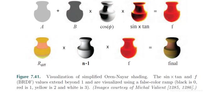
When the roughness is zero, the equation devolves to cdiff/π, the Lambertian BRDF, Equation 7.36. Oren and Nayar note that the 0.33 in the term for A can be replaced by 0.57 to better approximate surface interreflection. Valient [1285, 1286] presents techniques to rapidly evaluate this equation on the GPU. For a constant roughness, A and B can be precomputed. To compute cos(φ), the light and view vectors are projected to the surface’s tangent plane:

The resulting vectors are normalized, and the dot product of these vectors is then clamped to be non-negative, so computing the cos term. Valient converts the sin × tan term to a two-dimensional texture lookup, where the texture coordinates are n · l and n · v. Hoxley [314] gives a texture lookup version and a computed version.
In conclusion, although a large variety of analytic BRDF models exist in the literature, for most applications, a simple yet reasonably 合理的 expressive model such as the one in Equation 7.49 will suffice. In cases where a different BRDF is desired, pieces of models presented here can be added in a “mix-and-match” fashion to produce a new analytic BRDF. The Phong NDF can be extended to a sum of lobes, or an anisotropic NDF can be used [42, 43, 1326]. Alternatively, the Kajiya-Kay modification [620] 这个论文太模糊了,看不清 can be applied to convert an isotropic BRDF into an anisotropic one. The realism of the BRDF can be improved by incorporating visibility terms that change the behavior at glancing angles. The visibility term derived by Kelemen and Szirmay-Kalos [640] is particularly worthy of consideration due to its low cost and physical basis. The Lambertian diffuse term can be replaced with one that models the tradeoff between surface and body reflectance (see Section 7.5.4).
This “mixing and matching” can be extended to pieces represented as lookup tables, since they do not have an analytic closed-form expression. This might be because the values are manually painted for creative reasons. NDF maps are one possibility, but there are others. For example, a onedimensional lookup table could be used for the Fresnel term, to allow for hand-painted color shifts at glancing angles. In other cases, BRDF terms are derived by computing integrals that may not have closed-form solutions, such as the microfacet geometry term introduced by Ashikhmin et al. [41], or the reciprocal energy-conserving diffuse term introduced by Shirley et al. [640, 1170]. Incorporating such lookup tables can make a BRDF more expressive. However, a lookup table is not something we can modify by a parameter, so it cannot easily be made to vary over a surface.
the filed of possible BRDF models and representations is vast. we have endeavored to cover the options of most relevance to real-time rendering, but many others remain. interested readers are referred to the available surveys [44, 926, 1129, 1170, 1345, 1346], as well as the second volume of Glassner’s Principles of Digital Image Synthesis [409] and the more recent Digital Modeling of Material Appearance [275] by Dorsey, Rushmeier, and Sillion.
7.7 BRDF Acquisition and Representation 获取和表示
in most real-time applications, BRDFs are mannually selected and their parameters set to achieve a desired look. however, sometimes BRDFs are acquired, or measured, directly from actual surfaces. In some cases this is done to closely match rendered objects to real ones (digital doubles in film production, or digital reproductions of cultural artifacts). In others, it may be done to save authoring time. In either case, two problems need to be solved: how to capture the BRDF data, and once captured, how to represent it for later rendering.
7.7.1 acquiring BRDFs
Goniometers, imaging bidirectional reflectometers 双向反射测量, and image-based methods have been used to obtain the reflectance measurements over the incoming and outgoing angles. some of these databases are public and available online, such as those from Cornell University[200], Columbia-Utrecht [190], and MIT [871]. Ward [1326] discusses measurement in depth, Kautz et al. [630] give an overview of acquisition techniques, and Marschner et al.[821] discuss previous work and their own image-based method for measuring BRDFs, which has been since further refined by Matusik[825] and Ngan[926].
while the previously mentioned techniques measure a single BRDF function, the capture of spatially varying BRDFs (SVBRDFs) is of more interest, since real-world objects rarely have uniform reflectance. acquisition of SVBRDFS[225,226,1255] is an active area of research, especially from human faces[232,377,495] have been used in cmmercial applications [2,1096]. the columbia-utrecht database[190] includes some spatially variant measurements, as well as individual BRDFs.
7.7.2 Representations for Measured BRDFs
The result of a BRDF capture is a large, densely sampled four-dimensional table (six-dimensional for SVBRDFs). the acquisition process also unavoidlably introduces noise into the data. for these reasons, the raw data is unsuitable to be used directly for rendering——it must first be converted into some other representation[1089].
one common method is to select an analytic BRDF and fit its parameters to the measured data. this results in a very compact representation, and rendering is reasonably fast. the results are also easy to edit mannually if needed. however, it is not always simple to choose a BRDF for this purpose. the error introduced can be quite large and depends on the BRDF model chosen. one way to improve the quality of the results (although further complicating the fitting process) is to use a weighted sum of multiple BRDF terms, such as Ward[1326] or Blinn-Phong[97] lobes.
one model that was designed to be used in a multiple-term fitting process is the Laforturn BRDF [710], which generalizes the calcualtion of the reflection vector used in the original Phong model [1014]. this generation enables the modeling of retroreflective 回射 and anisotropic surfaces. McAllister et al. used multiple Lafortune terms to render SVBRDFs in real time on a GPU [830,831].
Ngan et al. [926] perform a detailed analysis of the errors introduced by fitting various measured materials to a selection of analytic BRDF models. for isotropic materials, Ward and Blinn-Phong BRDFs have the highest errors, most likely due to their lack of a Fresnel term (the original form of the Blinn-Phong BRDF was used, which does not have a Fresnel term). the Lafortune BRDF also has fairly high errors, evidently due to the fact that it is derived from a reflection-vector-based BRDF and shares the problems of that class of BRDF models (see section 7.5.7). the best results are achieved with the HTSG, Cook-Torrance, and Ashikhmin-Shirley BRDFs. about a third of the measured materials gained significant accuracy from the addition of a second lobe of the same type——one lobe was sufficient for the remainder.
Ngan et al. also analyzed several anisotropic materials. Only the Ward [1326] and Poulin-Fournier [1027] BRDFs were used for fitting. Both of them did moderately well on surfaces with simple anisotropic reflectance. Surfaces such as fabrics with complex, periodic microgeometry structure were not modeled well by any of the analytic BRDFs. For those materials, Ngan adopted an interesting semi-analytic fitting approach; an arbitrary microfacet distribution was deduced from the measurements, and then a BRDF was generated from the microfacet distribution, using the method introduced by Ashikhmin et al. [41]. This approach resulted in very good matches to the measured data.
Ashikhmin and Premoˇze propose [46] a distribution-based BRDF model that allows for extremely simple BRDF acquisition. A single image of a sample with known, curved geometry (taken with the light source and camera positions close to each other) can suffice to capture many materials.
Another way to represent BRDFs is to project them onto orthonormal bases, such as spherical harmonics [1344], spherical wavelets [180, 715, 1135], or Zernike Polynomials [681]. These techniques are focused on representing the shape of the BRDF as a generic function. Look again at Figure 7.17: For a given incoming direction, a surface is formed that represents the reflectance at any outgoing direction. The BRDF surface is generally changing in a smooth fashion, with few places where it changes rapidly. This implies that a sum of a few low- and high-frequency functions can capture the BRDF shape. Such projections are simpler to perform than fitting to a BRDF or sum of BRDF terms, as no optimization process is needed. However, many terms are usually needed to achieve a reasonable

match to the original function (dozens or hundreds), making these methods unsuitable for real-time rendering. Section 8.6.1 discusses basis projection in more detail.
7.8 Implementing BRDFs
to incorporate a BRDF model in a rendering system, the BRDF needs to be evaluated as part of a shading equation 反射方程. the purpose of a shading equation is to compute the outgoing radiance Lo from a surface location into the view direction v. given a set of n point or directional light sources, the outgoing radiance 出射反射率 is computed thus (repeating equation 7.2.1):

the cosine factor is computed as the clamped dot product between the surface normal and the kth light direction vector:

various methods for computing the value of Elk were discussed in section 7.4. the computation of the BRDF f(lk,v) remains in order to complete the evaluation of the shading equation.
As we have seen, most BRDFs contain a 1/π factor. In many rendering systems, this factor is folded into EL for convenience. When adapting a radiometrically defined BRDF (such as can be found in academic papers, or in Section 7.6 of this book) for use in such a rendering system, care must be taken to multiply the BRDF by π.
The most straightforward way to evaluate any BRDF model that has an analytic expression, as opposed to being represented by a factorization or a sum of basis functions, is to simply evaluate the expression in a shader for each light source (see Equation 7.21 on page 224). Evaluating the full expression in the pixel shader will give the best visual results, but in some cases slowly varying subexpressions can be evaluated in the vertex shader and interpolated. For spatially varying BRDFs, a common approach is to encode BRDF parameters in textures (see Section 6.5), although in some cases it might make sense to store them in vertices instead. 可以把BRDF的参数存储在纹理中,也可以存储在顶点中 Since evaluation of dot products is efficient on graphics hardware, BRDFs intended for realtime use are usually formulated in terms of cosines of angles between vectors such as the incoming light vector l, view vector v, half vector h, surface normal n, tangent t, or bitangent b. If both vectors are of length 1, the dot product is equal to the cosine of the angle between the vectors.
In principle, BRDF equations apply in the local frame of the surface defined by the vectors n, t, and b. In practice, they can be evaluated in
any coordinate system (or more than one) as long as care is taken never to perform an operation between vectors in different coordinate systems. Per-pixel BRDF evaluation is often combined with normal mapping 逐像素的BRDF计算通常和法线映射结合在一起使用. In principle, normal mapping perturbs the entire local frame, not just the normal. Isotropic BRDFs rarely require tangent or bitangent vectors, so perturbing the normal vector is sufficient. When shading with anisotropic BRDFs, it is important to perturb any tangent or bitangent vectors used. Anisotropic BRDFs introduce the possibility of per-pixel modification of the tangent direction—use of textures to perturb both the normal and tangent vectors is called frame mapping [618]. Frame mapping can enable effects such as brushed swirls on metal or curly hair. Some BRDFs are defined as a combination of subexpressions defined analytically and subexpressions defined by values stored in one- or twodimensional data tables (see Section 7.6). These semi-analytic BRDFs are computed much like fully analytic BRDFs, but with the addition of texture lookups for the tabulated subexpressions.
Even for fully analytically defined BRDFs, there might be a performance benefit in extracting a subexpression that is a function of one or two variables and tabulating its values in a texture for lookup while rendering. In the past, when computation was costly relative to texture lookups, this was a very common practice. Now computation is relatively cheap—a rule of thumb in 2007 was that one texture operation is equivalent to ten arithmetic operations (or more). 20 This number will keep growing as graphics hardware evolves [1400]. Only the most complex subexpressions will benefit from being factored into a texture. To avoid losing the parametric qualities of the BRDF, it is preferable for factored subexpressions to be independent of the BRDF’s parameters.
BRDFs using non-parametric representations are more difficult to render efficiently. In the case of BRDFs defined as an orthonormal expansion of bases such as spherical harmonics, rendering is straightforward—just evaluate the basis functions—but due to the large number of coefficients computation is likely to be expensive. More importantly, if the BRDF is spatially varying, then a very large number of texture reads is needed to read all of the coefficients, further reducing performance.
BRDFs that use factored representations are easier to render, since a relatively small number of textures are read (usually two). inverse Shade Trees [740] use a larger number of textures (about twenty for the examples given) but most of them are one dimensinal. this is still well within the capabilities of modern accelerators, but the large number of texture access will cause rendering of such BRDFs to be significantly slower than most analytic BRDFs. in addition, note that most of the texture access need to be repeated for each light source.
7.8.1 mipmapping BRDF and normap maps
in section 6.2, we discussed a problem with texture filtering: Mechanisms such as bilinear filtering and mipmapping are based on the assumption that the quanlity being filtered (which is an input to the shading equation) has a linear relationship to the final color (the output of the shading equation). although this is true for some quantities, such as diffuse and specular colorr, it is not true in general. artifacts can result from using linear mipmapping methods on normal maps, or on textures containing nonlinear BRDF parameters such as cosine powers. these artifacts can manifest aas flickering highlights, or as unexpected changes in surface gloss or brightness with a change in the surface’s distance from the camera.
to understand why these problems occur and how to solve them, it is important to remember that the BRDF is a statistical description of the effects of subpixel surface structure. when the distance between the camera and surface increases当摄像机和表面距离远的时候, surface structure that previously covered several pixels may be reduced to subpixel size, moving from the realm of bump maps into the realm of the BRDF. this transition is intimately tied to the mipmap chain, which encapsulates the reduction of texture details to subpixel size.
Let us consider how the appearance of an object such as the cylinder in Figure 7.44 is modeled for rendering. Appearance modeling always assumes a certain scale of observation. Macroscale (large scale) geometry is modeled as triangles, mesoscale 中尺度 (middle scale) geometry is modeled as textures, and microscale geometry, smaller than a single pixel, is modeled via the BRDF.
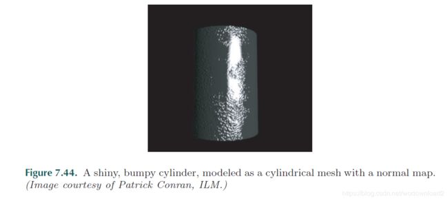
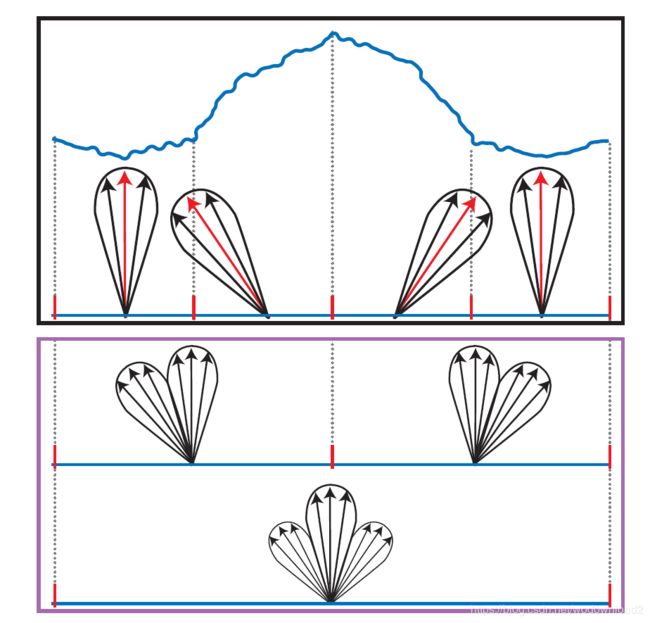
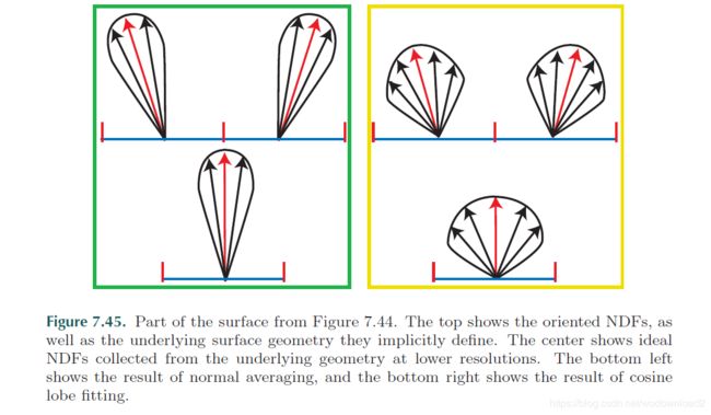
given the scale show in the image, it is appropriate to model the cylinder as a smooth mesh (macroscale), and represent the bumps with a normal map (mesoscale). a Blinn-Phong BRDF with a fixed cosine power is chosen to model the microscale normal distribution function (NDF). this combined representation models the cylinder apperance well at this scale. but what happens when the scale of observation changes?
study figure 7.45. the black-framed figurer at the top shows a small part of the surface, covered by four normal map texels. for each normal map texel, the normal is shown as a red arrow 红色箭头, surrounded by the cosine lobe NDF, show in black. the normals and NDF implicitly specify an underlying surface structure, which is shown in cross section. the large hump in the middle is one of the bumps from the normal map, and the small wiggles are the microscale surface structure. each texel in the normal map, combined with the cosine power, can bee seen as collecting the NDF across the surface area covered by the texel.
the idea representation of this surface at a lower resolution would exactly represent the NDFs collected across larger surface areas. the center of the figure (framed in purple) shows this idealized representation at half and one quarter of the original resolution. the gray dotted lines show which areas of the surface are covered by each texel. this idealized representation, if used for rendering, would most accurately represent the appearance of the surface at these lower resolutions.
in practice, the representation of the surface at low resolutions is the responsibility of the lower mipmap levels in the mipmap chain. at the bottom of the figure, we see two such sets of mipmap levels. on the bottom left (framed in green) we see the result of averaging and renormalizing the normals in the normal map, shown as NDFs oriented to the averaged normals. These NDFs do not resemble the ideal ones—they are pointing in the same direction, but they do not have the same shape. This will lead to the object not having the correct appearance. Worse, since these NDFs are so narrow, they will tend to cause aliasing, in the form of flickering highlights.
we can not represent the ideal NDFs directly with the Blinn-Phong BRDF. however, if we use a gloass map, the cosine power can be varied from texel to texel. let us imagine that, for each ideal NDF, we find the rotated cosine lobe that matches it most closely (both in orientation and overall width). we store the center direction of this cosine lobe in the normal map, and its cosine power in the gloass map. the results are shown on the bottom right (framed in yellow). these NDFs are much closer to the ideal ones. with this process, the appearance of the cylinder can be represented much more faithfully than with simple normal averaging, as can be seen in figure 7.46.

Figure 7.46. The cylinder from Figure 7.44. On the left, rendered with the original normal map. In the center, rendered with a much lower-resolution normal map containing averaged and renormalized normals (as shown in the bottom left of Figure 7.45). On the right, the cylinder is rendered with textures at the same low resolution, but containing normal and gloss values fitted to the ideal NDF, as shown in the bottom right of Figure 7.45. The image on the right is a significantly better representation of the original appearance. It will also be less prone to aliasing when rendered at low resolutions. (Image courtesy of Patrick Conran, ILM.)
in general, filtering normal maps in isolation will not produce the best results. the idea is to filter the entire surface appearance, represented by the BRDF, the normal map, and any other maps (gloass map, diffuse color map, specular color map, etc.). various methods have been developed to approximate this ideal.
Toksvig[1267] makes a clever observation, that if normals are averaged and not renormalized, the length of the averaged normal correlates inversely 和法线分布的宽度成反比 with the width of the normal distribution. that is, the more the original normals point in different directions, the shorter the normal averaged from them. assuming that a Blinn-Phong BRDF is used with cosine power m, Toksvig presents a method to compute a new cosine power m’. evaluating the Blinn-Phong BRDF with m’ instead of m approximates the spreading effect of the filtered normals. the equation for computing m’ is

where ||na|| is the length of the averaged normal. Toksvig’s method has the advantage of working with the most straightforward normal mipmapping scheme (linear averaging without normalization). this feature is particularly useful for dynamically generated normal maps (e.g., water ripples水波纹), for which mipmap generation must be done on the fly. 运行时 note that common methods of compressing normal maps require reconstructing the z-component from the other two, so they do not allow for non-unit-length normals. for this reason, normal maps used with Toksvig’s method may have to remain uncompressed. this issue can be partially compensated for by the ability to avoid storing a separate gloss map, as the normals in the normal map can be shortened to encode the gloss factor. Toksvig’s method does require a minor modification to the pixel shader to compute a gloss factor from the normal length. 运行时计算法线?
Conran at ILM[1911] proposes a process for computing the effect of filtered normal maps on specular response. 镜面反射的计算使用了过滤的法线贴图???the result representation is referred to as SpecVar maps. SpecVar map generation occurs in two stages.
第一阶段:高分辨率计算——evaluated at a high spatial resolution
in the first stage, the shading equation is evaluated at a high spatial resolution for a number of representative lighting 有代表性的光源和视觉方向 and viewing directions. the result is an array of shaded colors associated with each high-resolution surface location. each entry of this array is averaged across surface locations, producing an array of shaded colors for each low-resolution texel.
第二阶段:低分辨率拟合——fitting process
in the second stage a fitting process is performed at each low-resolution texel. the goal of the fitting process is to find the shading parameters that produce the cloest fit to the array values for the given lighting and viewing directions. these parameters are stored in texture maps, to be used during shading. although the details of the process are specific to Pixar’s RenderMan renderer, the algorithm can also be uesd to generate mipmap chains for real-time rendering. SpecVar map generation is computationally expensive, but it produces very high quality results. this method was used at ILM for effects shots in several feature films. figure 7.46 was also generated using this technique.
Schilling [1124] proposed storing three numbers at each location in the mipmap, to represent the variance of the normals in the u and v axes. unlike the previously discussed methods, this supports extracting anisotropic NDFs from the normal map. 从法线贴图中提取各向异性的NDFs Schilling describes an anisotropic variant of the Blinn-Phong BRDF using these three numbers. in later work [1125], this was extended to anisotropic shading with environment maps.
looking at the idea lowest-resolution 分辨率最低的 NDF in the middle of figure 7.45, we see three distinct lobes, 我们看到了3个不同的花瓣 which are only somewhat approximated by the single phong lobe on the bottom right. such multi-lobe NDFs appear when the normal map contains non-random structure. several approaches have been proposed to handle such cases. Tan et al. [1239,1240] and Han et al. [496] discuss methods to fit a mixture of multiple BRDF lobes to a filtered normal map. they demonstrate significant quality improvement over Toksvig’s method, but at the cost of considerable additional storage and shader computation. 但是时间和存储上更加耗费。
