OpenCV—python Gabor滤波(提取图像纹理)
文章目录
- 一、Gabor滤波简介
- 二、代码演示
Gabor是一个用于边缘提取的线性滤波器,其频率和方向表达与人类视觉系统类似,能够提供良好的方向选择和尺度选择特性,而且对于光照变化不敏感,因此十分适合纹理分析。在人脸识别等领域有着很广泛的应用
一、Gabor滤波简介
Gabor是一个用于边缘提取的线性滤波器,其频率和方向表达与人类视觉系统类似,能够提供良好的方向选择和尺度选择特性,而且对于光照变化不敏感,因此十分适合纹理分析。
Gabor滤波器和脊椎动物视觉皮层感受野响应的比较:第一行代表脊椎动物的视觉皮层感受野,第二行是Gabor滤波器,第三行是两者的残差。可见两者相差极小。Gabor滤波器的这一性质,使得其在视觉领域中经常被用来作图像的预处理。

Gabor滤波的公式如下所示:
g ( x , y ; λ , θ , ψ , σ , γ ) = exp ( − x ′ 2 + γ 2 y 2 2 σ 2 ) exp ( i ( 2 π x ′ λ + ψ ) ) g(x,y;λ,θ,ψ,σ,γ) = \exp(\frac{−x′^2+γ^2y^2}{2σ^2})\exp(i(2π\frac{x′}{λ}+ψ)) g(x,y;λ,θ,ψ,σ,γ)=exp(2σ2−x′2+γ2y2)exp(i(2πλx′+ψ))
其中实数部分与虚数部分为:
g r e a l ( x , y ; λ , θ , ψ , σ , γ ) = exp ( − x ′ 2 + γ 2 y 2 2 σ 2 ) cos ( 2 π x ′ λ + ψ ) g_{\rm real}(x,y;λ,θ,ψ,σ,γ)=\exp(\frac{−x′^2+γ^2y^2}{2σ^2})\cos(2π\frac{x′}{λ}+ψ) greal(x,y;λ,θ,ψ,σ,γ)=exp(2σ2−x′2+γ2y2)cos(2πλx′+ψ)
g i m a g ( x , y ; λ , θ , ψ , σ , γ ) = exp ( − x ′ 2 + γ 2 y 2 2 σ 2 ) sin ( 2 π x ′ λ + ψ ) g_{\rm imag}(x,y;λ,θ,ψ,σ,γ)=\exp(\frac{−x′^2+γ^2y^2}{2σ^2})\sin(2π\frac{x′}{λ}+ψ) gimag(x,y;λ,θ,ψ,σ,γ)=exp(2σ2−x′2+γ2y2)sin(2πλx′+ψ)
其中
{ x ′ = x c o s θ + y s i n θ y ′ = − x s i n θ + y c o s θ \left\{\begin{matrix} x′=xcosθ+ysinθ\\ y′=−xsinθ+ycosθ \end{matrix}\right. {x′=xcosθ+ysinθy′=−xsinθ+ycosθ
这里面的参数:
(1) x , y x,y x,y 分别表示像素坐标位置;
(2) λ λ λ 表示滤波的波长;(波长越大,黑白相间的间隔越大)
(3) θ θ θ 表示Gabor核函数图像的倾斜角度;
(4) ψ ψ ψ 表示相位偏移量,范围是-180~180;( ψ ψ ψ=0时白条为中心, ψ ψ ψ=180时,黑条为中心 )
(5) σ σ σ 表示高斯函数的标准差;( σ σ σ增大,条纹数量越多)
(6) γ γ γ 表示长宽比,决定这Gabor核函数图像的椭圆率。( γ γ γ越小,核函数图像会越高)
这里的参数不了解不要紧,后面我将会针对这些参数进行一系列的实验,直观的展示出这些参数的作用
| 参数 | 物理意义 | 描述 |
|---|---|---|
| x , y x,y x,y | 像素坐标位置 | |
| λ λ λ | 波长 | 直接影响滤波器的滤波尺度,通常大于等于2 |
| θ θ θ | 方向 | Gabor核函数图像的倾斜角度 |
| ψ ψ ψ | 相位偏移 | 调谐函数的相位偏移,取值 -180 ~ 180 |
| γ γ γ | 空间纵横比(长宽比) | 决定滤波器的形状椭圆率,取1时为圆形,通常取 0.5 |
| σ σ σ | 带宽 | 高斯滤波器的方差,通常取 2 π 2π 2π |
二、代码演示
import cv2,os
import numpy as np
import matplotlib.pyplot as plt
def get_img(input_Path):
img_paths = []
for (path, dirs, files) in os.walk(input_Path):
for filename in files:
if filename.endswith(('.jpg','.png')):
img_paths.append(path+'/'+filename)
return img_paths
#构建Gabor滤波器
def build_filters():
filters = []
ksize = [7,9,11,13,15,17] # gabor尺度,6个
lamda = np.pi/2.0 # 波长
for theta in np.arange(0, np.pi, np.pi / 4): #gabor方向,0°,45°,90°,135°,共四个
for K in range(6):
kern = cv2.getGaborKernel((ksize[K], ksize[K]), 1.0, theta, lamda, 0.5, 0, ktype=cv2.CV_32F)
kern /= 1.5*kern.sum()
filters.append(kern)
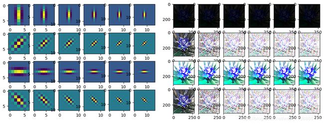
plt.figure(1)
#用于绘制滤波器
for temp in range(len(filters)):
plt.subplot(4, 6, temp + 1)
plt.imshow(filters[temp])
plt.show()
return filters
#Gabor特征提取
def getGabor(img,filters):
res = [] #滤波结果
for i in range(len(filters)):
# res1 = process(img, filters[i])
accum = np.zeros_like(img)
for kern in filters[i]:
fimg = cv2.filter2D(img, cv2.CV_8UC1, kern)
accum = np.maximum(accum, fimg, accum)
res.append(np.asarray(accum))
#用于绘制滤波效果
plt.figure(2)
for temp in range(len(res)):
plt.subplot(4,6,temp+1)
plt.imshow(res[temp], cmap='gray' )
plt.show()
return res #返回滤波结果,结果为24幅图,按照gabor角度排列
if __name__ == '__main__':
input_Path = './content'
filters = build_filters()
img_paths = get_img(input_Path)
for img in img_paths:
img = cv2.imread(img)
getGabor(img, filters)
这个过程有点慢,一张图片要1-3s,若是批量处理可以开启多线程,这样会快点
此代码用来查看滤波器
#coding:utf-8

'''
Gabor滤波器参数可视化
参考:https://blog.csdn.net/lhanchao/article/details/55006663
'''

import cv2
import numpy as np
import math

# λ(波长)变化
kernel1 = cv2.getGaborKernel((200,200),10,0,5,0.5,0)
kernel2 = cv2.getGaborKernel((200,200),10,0,10,0.5,0)
kernel3 = cv2.getGaborKernel((200,200),10,0,15,0.5,0)
kernel4 = cv2.getGaborKernel((200,200),10,0,20,0.5,0)

cv2.imshow("lambda: 5", kernel1)
cv2.imshow("lambda: 10", kernel2)
cv2.imshow("lambda: 15", kernel3)
cv2.imshow("lambda: 20", kernel4)

# θ变化
kernel1 = cv2.getGaborKernel((311, 311), 10, 0, 10, 0.5, 0)
kernel2 = cv2.getGaborKernel((311, 311), 10, math.pi * 0.25, 10, 0.5)
kernel3 = cv2.getGaborKernel((311, 311), 10, math.pi * 0.5, 10, 0.5, 0)
kernel4 = cv2.getGaborKernel((311, 311), 10, math.pi * 0.75, 10, 0.5, 0)

cv2.imshow("theta: 0", kernel1)
cv2.imshow("theta: 45", kernel2)
cv2.imshow("theta: 90", kernel3)
cv2.imshow("theta: 135", kernel4)

# ψ的变化

# σ的变化:
kernel1 = cv2.getGaborKernel((311, 311), 5, 0, 10, 0.5, 0)
kernel2 = cv2.getGaborKernel((311, 311), 10, 0, 10, 0.5, 0)
kernel3 = cv2.getGaborKernel((311, 311), 15, 0, 10, 0.5, 0)
kernel4 = cv2.getGaborKernel((311, 311), 20, 0, 10, 0.5, 0)

cv2.imshow("sigma: 5", kernel1)
cv2.imshow("sigma: 10", kernel2)
cv2.imshow("sigma: 15", kernel3)
cv2.imshow("sigma: 20", kernel4)

# γ的变化

kernel1 = cv2.getGaborKernel((200, 200), 10, 0, 10, 0.5, 0)
kernel2 = cv2.getGaborKernel((200, 200), 10, 0, 10, 1.0, 0)
kernel3 = cv2.getGaborKernel((200, 200), 10, 0, 10, 1.5, 0)
kernel4 = cv2.getGaborKernel((200, 200), 10, 0, 10, 2.0, 0)
cv2.imshow("gamma: 0.5", kernel1)
cv2.imshow("gamma: 1.0", kernel2)
cv2.imshow("gamma: 1.5", kernel3)
cv2.imshow("gamma: 2.0", kernel4)

cv2.waitKey()
cv2.destroyAllWindows()
未完待续
鸣谢
https://www.liangzl.com/get-article-detail-1703.html
https://blog.csdn.net/vitaminc4/article/details/78840904
https://blog.csdn.net/zizi7/article/details/53038031
https://blog.csdn.net/hanwenhui3/article/details/48289145
https://blog.csdn.net/sxlsxl119/article/details/81329266