入门神经网络优化算法（五）：一文看懂二阶优化算法Natural Gradient Descent（Fisher Information）

欢迎查看我的博客文章合集：我的Blog文章索引：：机器学习方法系列，深度学习方法系列，三十分钟理解系列等

这个系列会有多篇神经网络优化方法的复习/学习笔记，主要是一些优化器。目前有计划的包括：

• 入门神经网络优化算法（一）：Gradient Descent，Momentum，Nesterov accelerated gradient
• 入门神经网络优化算法（二）：Adaptive Optimization Methods：Adagrad，RMSprop，Adam
• 入门神经网络优化算法（三）：待定
• 入门神经网络优化算法（四）：AMSGrad，Radam等一些Adam变种
• 入门神经网络优化算法（五）：二阶优化算法Natural Gradient Descent（Fisher Information）
• 入门神经网络优化算法（六）：二阶优化算法K-FAC
• 入门神经网络优化算法（七）：二阶优化算法Shampoo

二阶优化算法Natural Gradient Descent，是从分布空间推导最速梯度下降方向的方法，和牛顿方法有非常紧密的联系。Fisher Information Matrix往往可以用来代替牛顿法的Hessian矩阵计算。下面详细道来。

1. Fisher Information Matrix

了解Natural Gradient Descent方法，需要先了解Fisher Information Matrix的定义。参考资料主要有[1][2]，加上我自己的理解。

1.1 Score function

假设我们有一个模型参数向量是$\theta$，似然函数一般表示成$p(x|\theta )$。在很多算法中，我们经常需要学习参数$\theta$以最大化似然函数（likelihood）$p(x|\theta )$。这个时候，定义Score function $s(\theta )$，the gradient of log likelihood function：
$$s(\theta )={\nabla }_{\theta }\log p(x|\theta )$$

这个Score function在很多地方都要用到，特别的，在强化学习Policy Gradient类方法中，我们会直接用到Score function求参数梯度来更新policy参数。

Score function的性质：The expected value of score function wrt. the model is zero.

证明：
$$\begin{gathered} E_{p(x|\theta )}\left[s(\theta )\right]=E_{p(x|\theta )}\left[\nabla \log p(x|\theta )\right] \\ =\int \nabla \log p(x|\theta )p(x|\theta )\text{d}x \\ =\int \frac{1}{p(x|\theta )}\nabla p(x|\theta )p(x|\theta )\text{d}x \\ =\int \nabla p(x|\theta )\text{d}x \\ =\nabla \int p(x|\theta )\text{d}x \\ =\nabla 1 \\ =0 \end{gathered}$$

1.2 Fisher Information

虽然期望为零，但是我们需要评估Score function的不确定性，我们采用协方差矩阵的期望（针对模型本身）：
$$E_{p(x|\theta )}\left[(s(\theta )-0)(s(\theta )-0{)}^{\text{T}}\right]$$
上述定义（协方差矩阵的期望，针对model $p(x|\theta )$ ）称之为Fisher Information，如果$\theta$是表示成一个列向量，那么Score function也是一个列向量，而Fisher Information是一个矩阵形式，我们称之为Fisher Information Matrix。

$$\text{F}=E_{p(x|\theta )}\left[\nabla \log p(x|\theta )\nabla \log p(x|\theta {)}^{\text{T}}\right]$$

但是呢，往往$p(x|\theta )$ 形式是比较复杂的，甚至是一个模型的输出，要计算期望是不太可能的。因此，实际上我们用的比较多的情况是，采用training data $X=\{x_1,x_2,\cdots ,x_N\}$计算得到的Empirical Fisher：
$$\text{F}=\frac{1}{N}\sum _{i=1}^N\nabla \log p(x_i|\theta )\nabla \log p(x_i|\theta {)}^{\text{T}}$$

1.3 Fisher矩阵和Hessian矩阵的关系

前面是背景介绍，下面进入正题，Fisher矩阵和Hessian矩阵的关系。可以证明：log似然函数的海森矩阵的期望的负数，等于Fisher Information Matrix.

Claim: The negative expected Hessian of log likelihood is equal to the Fisher Information Matrix F

证明：核心思想是，The Hessian of the log likelihood is given by the Jacobian of its gradient：
$$\begin{gathered} {\text{H}}_{\log p(x|\theta )}=\text{J}\left[\frac{\nabla p(x|\theta )}{p(x|\theta )}\right] \\ =\frac{{\text{H}}_{p(x|\theta )}p(x|\theta )-\nabla p(x|\theta )\nabla p(x|\theta {)}^{\text{T}}}{p(x|\theta )p(x|\theta )} \\ =\frac{{\text{H}}_{p(x|\theta )}p(x|\theta )}{p(x|\theta )p(x|\theta )}-\frac{\nabla p(x|\theta )\nabla p(x|\theta {)}^{\text{T}}}{p(x|\theta )p(x|\theta )} \\ =\frac{{\text{H}}_{p(x|\theta )}}{p(x|\theta )}-\left(\frac{\nabla p(x|\theta )}{p(x|\theta )}\right){\left(\frac{\nabla p(x|\theta )}{p(x|\theta )}\right)}^{\text{T}} \end{gathered}$$

推导的时候主要注意，$p(x|\theta )$是一个标量；而$\nabla p(x|\theta )$是对参数的梯度，是一个列向量。
然后Taking expectation wrt. the model, we have：

$$\begin{gathered} E_{p(x|\theta )}\left[{\text{H}}_{\log p(x|\theta )}\right]=E_{p(x|\theta )}\left[\frac{{\text{H}}_{p(x|\theta )}}{p(x|\theta )}-\left(\frac{\nabla p(x|\theta )}{p(x|\theta )}\right){\left(\frac{\nabla p(x|\theta )}{p(x|\theta )}\right)}^{\text{T}}\right] \\ =E_{p(x|\theta )}\left[\frac{{\text{H}}_{p(x|\theta )}}{p(x|\theta )}\right]-E_{p(x|\theta )}\left[\left(\frac{\nabla p(x|\theta )}{p(x|\theta )}\right){\left(\frac{\nabla p(x|\theta )}{p(x|\theta )}\right)}^{\text{T}}\right] \\ =\int \frac{{\text{H}}_{p(x|\theta )}}{p(x|\theta )}p(x|\theta )\text{d}x-E_{p(x|\theta )}\left[\nabla \log p(x|\theta )\nabla \log p(x|\theta {)}^{\text{T}}\right] \\ ={\text{H}}_{\int p(x|\theta )\text{d}x}-\text{F} \\ ={\text{H}}_1-\text{F} \\ =-\text{F}. \end{gathered}$$

因此我们得到了：$\text{F}=-E_{p(x|\theta )}\left[{\text{H}}_{\log p(x|\theta )}\right]$，证明完毕。我们可以将F的作用看作是对数似然函数曲率的度量。一种很自然的想法就是，在二阶优化算法中，比如牛顿法中，需要计算Hessian矩阵，那么是否可以用Fisher矩阵来代替Hessian举证呢？这就引出了下面要讲的natural gradient方法了。

2. 自然梯度下降法Natural Gradient Descent

先来讲一讲parameter space和distribution space的概念，导致了对梯度下降的不同理解。

• parameter space：一般我们解决优化问题最常用的方法是用梯度下降，每一步优化方向采用负梯度方向，$-{\nabla }_{\theta }\mathcal{L}(\theta )$。可以知道，负梯度方向是在当前的参数值$\theta$的local neighborhood里loss在参数空间的最速下降方向。
  $$\frac{-{\nabla }_{\theta }\mathcal{L}(\theta )}{\Vert {\nabla }_{\theta }\mathcal{L}(\theta )\Vert }=\underset{ϵ\to 0}{\lim }\frac{1}{ϵ}{\text{arg min}}_{d\text{ s.t. }\Vert d\Vert \le ϵ}\mathcal{L}(\theta +d).$$
  上面的表达式是，参数空间中最陡的下降方向是选取一个向量$d$，使得新参数$\theta +d$在当前参数$\theta$的$ϵ$-邻域内，并且我们选取使损失最小的$d$。注意我们用欧几里德范数来表示这个邻域。因此，梯度下降的优化依赖于参数空间的欧氏几何度量。

• distribution space：同时，如果我们的目标是最小化损失函数（最大化似然），那么我们自然会在所有可能的似然空间中采取优化步骤，通过参数$\theta$来实现。由于似然函数本身是一个概率分布，我们称它所在的空间为分布空间（distribution space）。因此，在分布空间中采用最陡下降方向，而不是参数空间，是有道理的。

在distribution space中，用什么距离度量呢？常用的选择就是用KL散度（KL-divergence），KL散度常用语评估两个分布的接近程度。但是，实际上KL散度是不对称的，因此理论上不是一个distance metric，但是呢，很多地方还是用KL散度来衡量两个分布的接近程度。（as $d$ goes to zero, KL-divergence is asymptotically symmetric. So, within a local neighbourhood, KL-divergence is approximately symmetric [3].）

2.1 分布空间中的最速下降，Natural gradient方法

前面讲了那么多，终于要引出自然梯度方法的基本推导了。

先推导KL散度的泰勒展开有如下形式：
$$\text{KL}[p(x|\theta )\Vert p(x|\theta +d)]\approx \frac{1}{2}{d}^{\text{T}}\text{F}d$$

证明：写出二阶泰勒展开：

$$\begin{gathered} \text{KL}[p(x|\theta )\Vert p(x|\theta +d)] \\ \approx \text{KL}[p(x|\theta )\Vert p(x|{\theta }^{\prime })]{|}_{{\theta }^{\prime }=\theta }+({{\nabla }_{{\theta }^{\prime }}\text{KL}[p(x|\theta )\Vert p(x|{\theta }^{\prime })]|}_{{\theta }^{\prime }=\theta }{)}^{\text{T}}d+\frac{1}{2}{d}^{\text{T}}{\nabla }_{{\theta }^{\prime }}^2\text{KL}[p(x|\theta )\Vert p(x|{\theta }^{\prime })]{|}_{{\theta }^{\prime }=\theta }d \\ =\text{KL}[p(x|\theta )\Vert p(x|\theta )]-E_{p(x|\theta )}[{\nabla }_{\theta }\log p(x|\theta ){]}^{\text{T}}d+\frac{1}{2}{d}^{\text{T}}\text{F}d=\frac{1}{2}{d}^{\text{T}}\text{F}d \end{gathered}$$

这样理解为什么引入${\theta }^{\prime }$：把KL散度第一个$p(x|\theta )$看成一个确定的分布，而变化的是在第二个分布的参数上。我们依次来看下约等号$\approx$后面这三项：

• 泰勒展开的第一项 $\text{KL}[p_{\theta }\Vert p_{\theta }]=0$

• 第二项的推导：
  $$\begin{gathered} {\nabla }_{{\theta }^{\prime }}\text{KL}[p(x|\theta )\Vert p(x|{\theta }^{\prime })]={\nabla }_{{\theta }^{\prime }}{E}_{p(x|\theta )}[\log p(x|\theta )]-{\nabla }_{{\theta }^{\prime }}{E}_{p(x|\theta )}[\log p(x|{\theta }^{\prime })] \\ =-E_{p(x|\theta )}[{\nabla }_{{\theta }^{\prime }}\log p(x|{\theta }^{\prime })]=0 \end{gathered}$$
  考虑${|}_{{\theta }^{\prime }=\theta }$的话，第二项包含了Score function的期望。正好是本章节前面Fisher Matrix部分讲过的，Score function的期望，已经证明过是0。

• 第三项，需要用到前面第一章证明过的，$\text{F}=-E_{p(x|\theta )}\left[{\text{H}}_{\log p(x|\theta )}\right]$，以及如下性质：Fisher Information Matrix F is the Hessian of KL-divergence between two distributions $p(x|\theta )$ and $p(x|{\theta }^{\prime })$, with respect to ${\theta }^{\prime }$, evaluated at ${\theta }^{\prime }=\theta$，下面是推导过程：
  $$\text{KL}[p(x|\theta )\Vert p(x|{\theta }^{\prime })]=E_{p(x|\theta )}[\log p(x|\theta )]-E_{p(x|\theta )}[\log p(x|{\theta }^{\prime })]$$
  The first derivative wrt. ${\theta }^{\prime }$ is：
  $$\begin{gathered} {\nabla }_{{\theta }^{\prime }}\text{KL}[p(x|\theta )\Vert p(x|{\theta }^{\prime })]={\nabla }_{{\theta }^{\prime }}{E}_{p(x|\theta )}[\log p(x|\theta )]-{\nabla }_{{\theta }^{\prime }}{E}_{p(x|\theta )}[\log p(x|{\theta }^{\prime })] \\ =-E_{p(x|\theta )}[{\nabla }_{{\theta }^{\prime }}\log p(x|{\theta }^{\prime })] \\ =-\int p(x|\theta ){\nabla }_{{\theta }^{\prime }}\log p(x|{\theta }^{\prime })\text{d}x \end{gathered}$$
  The second derivative is：
  $$\begin{gathered} {\nabla }_{{\theta }^{\prime }}^2\text{KL}[p(x|\theta )\Vert p(x|{\theta }^{\prime })]{|}_{{\theta }^{\prime }=\theta }=-\int p(x|\theta ){\nabla }_{{\theta }^{\prime }}^2\log p(x|{\theta }^{\prime }){|}_{{\theta }^{\prime }=\theta }\text{d}x \\ =-\int p(x|\theta ){\text{H}}_{\log p(x|\theta )}\text{d}x \\ =-E_{p(x|\theta )}[{\text{H}}_{\log p(x|\theta )}] \\ =\text{F} \end{gathered}$$

所以得到KL散度的二阶泰勒展开形式：
$$\text{KL}[p(x|\theta )\Vert p(x|\theta +d)]\approx \frac{1}{2}{d}^{\text{T}}\text{F}d$$

现在，我们想知道什么是使分布空间中的损失函数L最小化的更新向量d，以便我们知道哪个方向的KL散度减小得最多。这类似于最速下降法，但在以KL散度为度量的分布空间，而不是通常的以欧氏度量的参数空间。为此，我们将最小化：

$$d^{\ast }={\text{arg min}}_{d\text{ s.t. }\text{KL}[p_{\theta }\Vert p_{\theta +d}]\le c}\mathcal{L}(\theta +d),$$

如果我们写出上面的最小化问题在拉格朗日乘子法形式，用二阶泰勒展开近似KL散度，用一阶泰勒级数展开近似$\mathcal{L}$：

$$\begin{gathered} d^{\ast }={\text{arg min}}_d\mathcal{L}(\theta +d)+\lambda (\text{KL}[p_{\theta }\Vert p_{\theta +d}]-c) \\ \approx {\text{arg min}}_d\mathcal{L}(\theta )+{\nabla }_{\theta }\mathcal{L}(\theta {)}^{\text{T}}d+\frac{1}{2}\lambda d^{\text{T}}\text{F}d-\lambda c \end{gathered}$$
其中$\lambda$是拉格朗日系数，要求解这个优化问题，我们求$d$的梯度等于0：
$$\begin{gathered} 0=\frac{\partial }{\partial d}\left[\mathcal{L}(\theta )+{\nabla }_{\theta }\mathcal{L}(\theta {)}^{\text{T}}d+\frac{1}{2}\lambda d^{\text{T}}\text{F}d-\lambda c\right] \\ ={\nabla }_{\theta }\mathcal{L}(\theta )+\lambda \text{F}d \\ \lambda \text{F}d=-{\nabla }_{\theta }\mathcal{L}(\theta ) \\ d=-\frac{1}{\lambda }{\text{F}}^{-1}{\nabla }_{\theta }\mathcal{L}(\theta ) \end{gathered}$$

因此，先不看$\frac{1}{\lambda }$（可以一起考虑吸收到learning rate部分），我们得到在分布空间中，最优的更新方向是$-{\text{F}}^{-1}{\nabla }_{\theta }\mathcal{L}(\theta )$。（类比二阶优化方法的牛顿法，更新方向是$-{\text{H}}^{-1}{\nabla }_{\theta }\mathcal{L}(\theta )$，非常类似吧）。

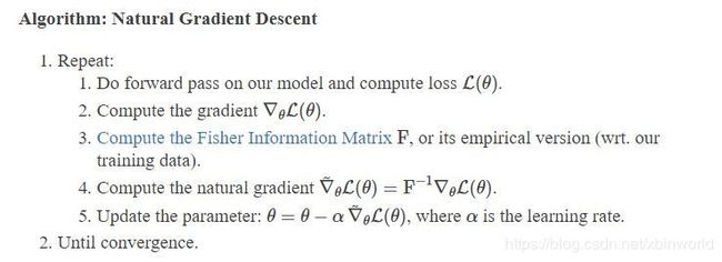
我们把Natural gradient 定义成：${\tilde{\nabla }}_{\theta }\mathcal{L}(\theta )={\text{F}}^{-1}{\nabla }_{\theta }\mathcal{L}(\theta )$. 自然梯度下降算法的基本流程如下：（一般我们会采用batch模式的Empirical Fisher Matrix：$\text{F}=\frac{1}{N}{\sum }_{i=1}^N\nabla \log p(x_i|\theta )\nabla \log p(x_i|\theta {)}^{\text{T}}$）

与Adam关系的类比讨论

在数据量较少的非常简单的模型中，我们看到可以很容易地实现自然梯度下降。但众所周知，深度学习模型中的参数数目非常大，千万甚至亿级参数量模型很常见，即使一层都有上百万参数。这类模型的Fisher信息矩阵难以计算、存储、以及求逆。这和二阶优化方法在深度学习中不受欢迎的原因是一样的。

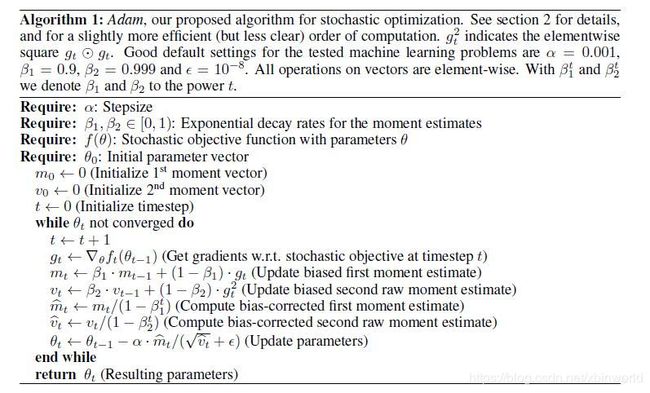
解决这个问题的一种方法是计算近似的Fisher/Hessian。像ADAM[5]这样的方法计算梯度的一阶和二阶moving average（m和v）。m是动量momentum，这里不讨论。而v可以看成是Fisher信息矩阵的近似——但将其约束为对角矩阵（协方差的对角线元素是梯度的平方）。因此，在ADAM中，我们只需要$O(n)$空间来存储（F的近似值）而不是$O(n^2)$，并且可以在$O(n)$而不是$O(n^3)$中进行求逆运算。在实践中，ADAM工作得非常好，是目前优化深层神经网络的基准优化方法。

OK，这一篇终于基本写好了，后面会继续这个话题，再记录一下如何加速自然梯度方法的工作，主要是比较知名的K-FAC算法。这篇可能还有一些关于自然梯度的引申讨论，过几天再补。参考[6][7]。TBD…

参考资料

[1] https://wiseodd.github.io/techblog/2018/03/11/fisher-information/
[2] https://wiseodd.github.io/techblog/2018/03/14/natural-gradient/
[3] Martens, James. “New insights and perspectives on the natural gradient method.” arXiv preprint arXiv:1412.1193 (2014).
[4] Ly, Alexander, et al. “A tutorial on Fisher information.” Journal of Mathematical Psychology 80 (2017): 40-55
[5] ADAM A METHOD FOR STOCHASTIC OPTIMIZATION. 2015
[6] 多角度理解自然梯度，https://zhuanlan.zhihu.com/p/82934100
[7] 如何理解 natural gradient descent?，https://www.zhihu.com/question/266846405