04_行销(Marketing)中的产品分析 (Product Analytics)
产品分析
- Load packages
- Load the dataset
- Product Analytics
我们将切换对客户行为进行分析的方式,并开始讨论如何使用数据科学进行更精细的产品级分析。越来越多的公司(尤其是电子商务企业)对利用数据来了解客户如何与不同产品互动和互动的兴趣和需求不断增加。业已证明,严格的产品分析可以帮助企业改善用户参与度和转化率,从而最终带来更高的利润。在本章中,我们将讨论什么是产品分析以及如何将其用于不同的用例。
产品分析是一种从数据中获取见解的方法,这些数据涉及客户如何与所提供的产品互动和互动,不同产品的性能如何以及企业中可观察到的某些弱点和优势。但是,产品分析并不仅限于分析数据。产品分析的最终目的实际上是建立可行的见解和报告,这些信息和报告可以进一步帮助优化和改善产品性能,并根据产品分析的结果生成新的营销或产品创意。产品分析从跟踪事件开始。这些事件可以是客户的网站访问,页面浏览量,浏览器历史记录,购买或客户可以对您提供的产品采取的任何其他操作。然后,我们可以开始分析和可视化这些事件中的任何可观察模式,以创建可行的见解或报告为目标。产品分析的一些共同目标如下:
- 提高客户和产品保留率
通过分析查看和购买的客户,可以确定客户重复购买的商品以及那些重复的顾客。另一方面,您还可以确定客户不购买哪些商品以及有搅动风险的客户。分析和了解重复购买的商品和回头客的共同属性可以帮助您改善保留策略。 - 识别流行和趋势产品
作为零售企业的营销商,重要的是要对流行和趋势产品有很好的了解。这些最畅销的产品是业务的主要收入来源,并提供了新的销售机会,例如交叉销售或捆绑销售。借助产品分析,就能够轻松地识别和跟踪这些流行和流行的产品,并使用这些最畅销的产品生成新的战略来探索不同的机会。 - 根据客户和产品的关键属性对客户和产品进行细分
借助客户资料和产品数据,我们可以使用产品分析根据客户和产品的属性对客户群和产品进行细分。细分产品数据的一些方法是基于它们的盈利能力,销售量,重新订购量和退款数量。通过这些细分,可以得出关于下一步要定位的产品或客户细分的可行见解。 - 制定具有更高ROI的营销策略
产品分析还可以用于分析营销策略的投资回报率(ROI)。通过分析在促销某些项目上花费的营销费用以及从这些产品产生的收入,可以了解什么有效,哪些无效。使用产品分析进行营销ROI分析可以帮助创建更有效的营销策略
在这篇文章里,我会使用一个在线零售的数据集,仍然是来自Kaggle,数据集是OnlineRetail.csv 。我们将讨论如何跟踪流行商品随时间变化的趋势,然后简要讨论如何在营销策略中如何利用这种流行商品数据进行产品推荐。
# This Python 3 environment comes with many helpful analytics libraries installed
# It is defined by the kaggle/python Docker image: https://github.com/kaggle/docker-python
# For example, here's several helpful packages to load

import numpy as np # linear algebra
import pandas as pd # data processing, CSV file I/O (e.g. pd.read_csv)

# Input data files are available in the read-only "../input/" directory
# For example, running this (by clicking run or pressing Shift+Enter) will list all files under the input directory

import os
for dirname, _, filenames in os.walk('/kaggle/input'):
    for filename in filenames:
        print(os.path.join(dirname, filename))

# You can write up to 5GB to the current directory (/kaggle/working/) that gets preserved as output when you create a version using "Save & Run All"
# You can also write temporary files to /kaggle/temp/, but they won't be saved outside of the current session
/kaggle/input/onlineretail/OnlineRetail.csv
Load packages
import matplotlib.pyplot as plt
import pandas as pd
%matplotlib inline
Load the dataset
df=pd.read_csv(r"../input/onlineretail/OnlineRetail.csv", encoding="cp1252")
df.head(3)
| InvoiceNo | StockCode | Description | Quantity | InvoiceDate | UnitPrice | CustomerID | Country | |
|---|---|---|---|---|---|---|---|---|
| 0 | 536365 | 85123A | WHITE HANGING HEART T-LIGHT HOLDER | 6 | 12/1/2010 8:26 | 2.55 | 17850.0 | United Kingdom |
| 1 | 536365 | 71053 | WHITE METAL LANTERN | 6 | 12/1/2010 8:26 | 3.39 | 17850.0 | United Kingdom |
| 2 | 536365 | 84406B | CREAM CUPID HEARTS COAT HANGER | 8 | 12/1/2010 8:26 | 2.75 | 17850.0 | United Kingdom |
df.dtypes
InvoiceNo       object
StockCode       object
Description     object
Quantity         int64
InvoiceDate     object
UnitPrice      float64
CustomerID     float64
Country         object
dtype: object
Product Analytics
Quantity Distribution
ax = df['Quantity'].plot.box(
    showfliers=False,
    grid=True,
    figsize=(10, 7)
)

ax.set_ylabel('Order Quantity')
ax.set_title('Quantity Distribution')

plt.suptitle("")
plt.show()

pd.DataFrame(df['Quantity'].describe())
| Quantity | |
|---|---|
| count | 541909.000000 |
| mean | 9.552250 |
| std | 218.081158 |
| min | -80995.000000 |
| 25% | 1.000000 |
| 50% | 3.000000 |
| 75% | 10.000000 |
| max | 80995.000000 |
As you can see from this plot, some orders have negative quantities. This is because the cancelled or refunded orders are recorded with negative values in the Quantity column of our dataset. For illustration purposes in this exercise, we are going to disregard the cancelled orders.
df = df.loc[df['Quantity'] > 0]
Time-series Number of Orders
df['InvoiceDate']=pd.to_datetime(df.InvoiceDate)
monthly_orders_df = df.set_index('InvoiceDate')['InvoiceNo'].resample('M').nunique()
monthly_orders_df
InvoiceDate
2010-12-31    1629
2011-01-31    1120
2011-02-28    1126
2011-03-31    1531
2011-04-30    1318
2011-05-31    1731
2011-06-30    1576
2011-07-31    1540
2011-08-31    1409
2011-09-30    1896
2011-10-31    2129
2011-11-30    2884
2011-12-31     839
Freq: M, Name: InvoiceNo, dtype: int64
ax = pd.DataFrame(monthly_orders_df.values).plot(
    grid=True,
    figsize=(10,7),
    legend=False
)

ax.set_xlabel('date')
ax.set_ylabel('number of orders/invoices')
ax.set_title('Total Number of Orders Over Time')

plt.xticks(
    range(len(monthly_orders_df.index)),
    [x.strftime('%m.%Y') for x in monthly_orders_df.index],
    rotation=45
)

plt.show()
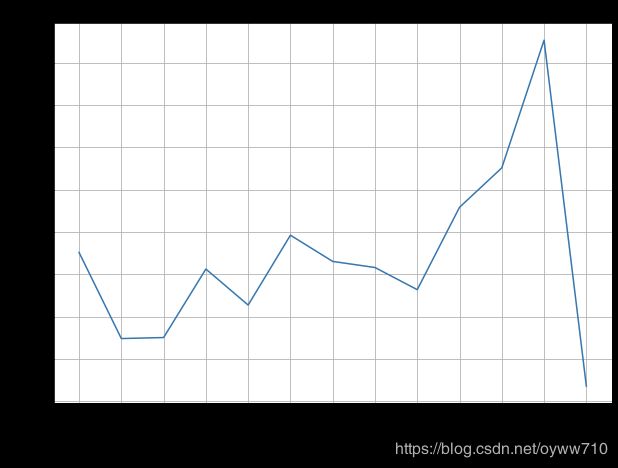
there is a sudden radical drop in the number of orders in December 2011. If you look closely at the data, this is simply because we do not have the data for the full month of December 2011. We can verify this by using the following code
invoice_dates = df.loc[
    df['InvoiceDate'] >= '2011-12-01',
    'InvoiceDate'
]

print('Min date: %s\nMax date: %s' % (invoice_dates.min(), invoice_dates.max()))
Min date: 2011-12-01 08:33:00
Max date: 2011-12-09 12:50:00
df = df.loc[df['InvoiceDate'] < '2011-12-01']
monthly_orders_df = df.set_index('InvoiceDate')['InvoiceNo'].resample('M').nunique()
ax = pd.DataFrame(monthly_orders_df.values).plot(
    grid=True,
    figsize=(10,7),
    legend=False
)

ax.set_xlabel('date')
ax.set_ylabel('number of orders')
ax.set_title('Total Number of Orders Over Time')

ax.set_ylim([0, max(monthly_orders_df.values)+500])

plt.xticks(
    range(len(monthly_orders_df.index)),
    [x.strftime('%m.%Y') for x in monthly_orders_df.index],
    rotation=45
)

plt.show()

Time-series Revenue
df['Sales'] = df['Quantity'] * df['UnitPrice']
monthly_revenue_df = df.set_index('InvoiceDate')['Sales'].resample('M').sum()
monthly_revenue_df
InvoiceDate
2010-12-31     823746.140
2011-01-31     691364.560
2011-02-28     523631.890
2011-03-31     717639.360
2011-04-30     537808.621
2011-05-31     770536.020
2011-06-30     761739.900
2011-07-31     719221.191
2011-08-31     737014.260
2011-09-30    1058590.172
2011-10-31    1154979.300
2011-11-30    1509496.330
Freq: M, Name: Sales, dtype: float64
ax = pd.DataFrame(monthly_revenue_df.values).plot(
    grid=True,
    figsize=(10,7),
    legend=False
)

ax.set_xlabel('date')
ax.set_ylabel('sales')
ax.set_title('Total Revenue Over Time')

ax.set_ylim([0, max(monthly_revenue_df.values)+100000])

plt.xticks(
    range(len(monthly_revenue_df.index)),
    [x.strftime('%m.%Y') for x in monthly_revenue_df.index],
    rotation=45
)

plt.show()

time-series Repeat Customers
invoice_customer_df = df.groupby(
    by=['InvoiceNo', 'InvoiceDate']
).agg({
    'Sales': sum,
    'CustomerID': max,
    'Country': max,
}).reset_index()
invoice_customer_df.head()
| InvoiceNo | InvoiceDate | Sales | CustomerID | Country | |
|---|---|---|---|---|---|
| 0 | 536365 | 2010-12-01 08:26:00 | 139.12 | 17850.0 | United Kingdom |
| 1 | 536366 | 2010-12-01 08:28:00 | 22.20 | 17850.0 | United Kingdom |
| 2 | 536367 | 2010-12-01 08:34:00 | 278.73 | 13047.0 | United Kingdom |
| 3 | 536368 | 2010-12-01 08:34:00 | 70.05 | 13047.0 | United Kingdom |
| 4 | 536369 | 2010-12-01 08:35:00 | 17.85 | 13047.0 | United Kingdom |
monthly_repeat_customers_df = invoice_customer_df.set_index('InvoiceDate').groupby([
    pd.Grouper(freq='M'), 'CustomerID'
]).filter(lambda x: len(x) > 1).resample('M').nunique()['CustomerID']

monthly_repeat_customers_df
InvoiceDate
2010-12-31    263
2011-01-31    153
2011-02-28    153
2011-03-31    203
2011-04-30    170
2011-05-31    281
2011-06-30    220
2011-07-31    227
2011-08-31    198
2011-09-30    272
2011-10-31    324
2011-11-30    541
Freq: M, Name: CustomerID, dtype: int64
Let’s take a closer look at the groupby function in this code. Here, we group by two conditions???pd.Grouper(freq=‘M’) and CustomerID. The first groupby condition, pd.Grouper(freq=‘M’), groups the data by the index, InvoiceDate, into each month. Then, we group this data by each CustomerID. Using the filter function, we can subselect the data by a custom rule. Here, the filtering rule, lambda x: len(x) > 1, means we want to retrieve those with more than one record in the group. In other words, we want to retrieve only those customers with more than one order in a given month. Lastly, we resample and aggregate by each month and count the number of unique customers in each month by using resample(‘M’) and nunique
monthly_unique_customers_df = df.set_index('InvoiceDate')['CustomerID'].resample('M').nunique()
monthly_unique_customers_df
InvoiceDate
2010-12-31     886
2011-01-31     742
2011-02-28     759
2011-03-31     975
2011-04-30     857
2011-05-31    1057
2011-06-30     992
2011-07-31     950
2011-08-31     936
2011-09-30    1267
2011-10-31    1365
2011-11-30    1666
Freq: M, Name: CustomerID, dtype: int64
monthly_repeat_percentage = monthly_repeat_customers_df/monthly_unique_customers_df*100.0
monthly_repeat_percentage
InvoiceDate
2010-12-31    29.683973
2011-01-31    20.619946
2011-02-28    20.158103
2011-03-31    20.820513
2011-04-30    19.836639
2011-05-31    26.584674
2011-06-30    22.177419
2011-07-31    23.894737
2011-08-31    21.153846
2011-09-30    21.468035
2011-10-31    23.736264
2011-11-30    32.472989
Freq: M, Name: CustomerID, dtype: float64
ax = pd.DataFrame(monthly_repeat_customers_df.values).plot(
    figsize=(10,7)
)

pd.DataFrame(monthly_unique_customers_df.values).plot(
    ax=ax,
    grid=True
)


ax2 = pd.DataFrame(monthly_repeat_percentage.values).plot.bar(
    ax=ax,
    grid=True,
    secondary_y=True,
    color='green',
    alpha=0.2
)

ax.set_xlabel('date')
ax.set_ylabel('number of customers')
ax.set_title('Number of All vs. Repeat Customers Over Time')

ax2.set_ylabel('percentage (%)')

ax.legend(['Repeat Customers', 'All Customers'])
ax2.legend(['Percentage of Repeat'], loc='upper right')

ax.set_ylim([0, monthly_unique_customers_df.values.max()+100])
ax2.set_ylim([0, 100])

plt.xticks(
    range(len(monthly_repeat_customers_df.index)),
    [x.strftime('%m.%Y') for x in monthly_repeat_customers_df.index],
    rotation=45
)

plt.show()

Revenue from Repeat Customers
monthly_rev_repeat_customers_df = invoice_customer_df.set_index('InvoiceDate').groupby([
    pd.Grouper(freq='M'), 'CustomerID'
]).filter(lambda x: len(x) > 1).resample('M').sum()['Sales']
monthly_rev_perc_repeat_customers_df = monthly_rev_repeat_customers_df/monthly_revenue_df * 100.0
monthly_rev_repeat_customers_df
InvoiceDate
2010-12-31    359170.60
2011-01-31    222124.00
2011-02-28    191229.37
2011-03-31    267390.48
2011-04-30    195474.18
2011-05-31    378197.04
2011-06-30    376307.26
2011-07-31    317475.00
2011-08-31    317134.25
2011-09-30    500663.36
2011-10-31    574006.87
2011-11-30    713775.85
Freq: M, Name: Sales, dtype: float64
ax = pd.DataFrame(monthly_revenue_df.values).plot(figsize=(12,9))

pd.DataFrame(monthly_rev_repeat_customers_df.values).plot(
    ax=ax,
    grid=True,
)

ax.set_xlabel('date')
ax.set_ylabel('sales')
ax.set_title('Total Revenue vs. Revenue from Repeat Customers')

ax.legend(['Total Revenue', 'Repeat Customer Revenue'])

ax.set_ylim([0, max(monthly_revenue_df.values)+100000])

ax2 = ax.twinx()

pd.DataFrame(monthly_rev_perc_repeat_customers_df.values).plot(
    ax=ax2,
    kind='bar',
    color='g',
    alpha=0.2
)

ax2.set_ylim([0, max(monthly_rev_perc_repeat_customers_df.values)+30])
ax2.set_ylabel('percentage (%)')
ax2.legend(['Repeat Revenue Percentage'])

ax2.set_xticklabels([
    x.strftime('%m.%Y') for x in monthly_rev_perc_repeat_customers_df.index
])

plt.show()

Popular Items Over Time
date_item_df = pd.DataFrame(
    df.set_index('InvoiceDate').groupby([
        pd.Grouper(freq='M'), 'StockCode'
    ])['Quantity'].sum()
)
date_item_df.head()
| Quantity | ||
|---|---|---|
| InvoiceDate | StockCode | |
| 2010-12-31 | 10002 | 251 |
| 10120 | 16 | |
| 10123C | 1 | |
| 10124A | 4 | |
| 10124G | 5 |
# Rank items by the last month sales
last_month_sorted_df = date_item_df.loc['2011-11-30'].sort_values(
    by='Quantity', ascending=False
).reset_index()

last_month_sorted_df
| InvoiceDate | StockCode | Quantity | |
|---|---|---|---|
| 0 | 2011-11-30 | 23084 | 14954 |
| 1 | 2011-11-30 | 84826 | 12551 |
| 2 | 2011-11-30 | 22197 | 12460 |
| 3 | 2011-11-30 | 22086 | 7908 |
| 4 | 2011-11-30 | 85099B | 5909 |
| ... | ... | ... | ... |
| 2941 | 2011-11-30 | 17129F | 1 |
| 2942 | 2011-11-30 | 85049c | 1 |
| 2943 | 2011-11-30 | 85114b | 1 |
| 2944 | 2011-11-30 | 85129C | 1 |
| 2945 | 2011-11-30 | 35913B | 1 |
2946 rows ?? 3 columns
# Regroup for top 5 items
date_item_df = pd.DataFrame(
    df.loc[
        df['StockCode'].isin(['23084', '84826', '22197', '22086', '85099B'])
    ].set_index('InvoiceDate').groupby([
        pd.Grouper(freq='M'), 'StockCode'
    ])['Quantity'].sum()
)
date_item_df
| Quantity | ||
|---|---|---|
| InvoiceDate | StockCode | |
| 2010-12-31 | 85099B | 2152 |
| 2011-01-31 | 85099B | 2747 |
| 2011-02-28 | 85099B | 3080 |
| 2011-03-31 | 85099B | 5282 |
| 2011-04-30 | 85099B | 2456 |
| 2011-05-31 | 85099B | 3621 |
| 2011-06-30 | 85099B | 3682 |
| 2011-07-31 | 85099B | 3129 |
| 2011-08-31 | 85099B | 5502 |
| 2011-09-30 | 85099B | 4401 |
| 2011-10-31 | 85099B | 5412 |
| 2011-11-30 | 85099B | 5909 |
trending_itmes_df = date_item_df.reset_index().pivot('InvoiceDate','StockCode').fillna(0)

trending_itmes_df = trending_itmes_df.reset_index()
trending_itmes_df = trending_itmes_df.set_index('InvoiceDate')
trending_itmes_df.columns = trending_itmes_df.columns.droplevel(0)

trending_itmes_df
| StockCode | 85099B |
|---|---|
| InvoiceDate | |
| 2010-12-31 | 2152 |
| 2011-01-31 | 2747 |
| 2011-02-28 | 3080 |
| 2011-03-31 | 5282 |
| 2011-04-30 | 2456 |
| 2011-05-31 | 3621 |
| 2011-06-30 | 3682 |
| 2011-07-31 | 3129 |
| 2011-08-31 | 5502 |
| 2011-09-30 | 4401 |
| 2011-10-31 | 5412 |
| 2011-11-30 | 5909 |
ax = pd.DataFrame(trending_itmes_df.values).plot(
    figsize=(10,7),
    grid=True,
)

ax.set_ylabel('number of purchases')
ax.set_xlabel('date')
ax.set_title('Item Trends over Time')

ax.legend(trending_itmes_df.columns, loc='upper left')

plt.xticks(
    range(len(trending_itmes_df.index)),
    [x.strftime('%m.%Y') for x in trending_itmes_df.index],
    rotation=45
)

plt.show()
