09_行销（Marketing）里数据驱动的客户细分

在营销中，我们经常尝试了解客户群某些子群体的行为。尤其是在有针对性的营销中，营销人员试图以某种方式细分客户群，并专注于每个目标细分市场或客户群。由于目标客户群中那些客户的需求和兴趣与企业的产品，服务或内容保持一致并更好地匹配，因此集中于某些目标客户群可以带来更好的绩效。鉴于当今市场上的竞争，了解客户的不同行为，类型和兴趣至关重要。尤其是在有针对性的营销中，对客户进行了解和分类是形成有效营销策略的重要步骤。通过细分客户群，营销人员可以一次专注于一个客户群。它还可以帮助营销人员一次针对一个特定的受众量身定制营销信息。客户细分是成功进行有针对性的营销的基础，通过该细分，您可以以不同的定价选项，促销和产品放置来针对特定的客户群，从而以最具成本效益的方式吸引目标受众的兴趣。

聚类算法通常在市场营销中用于客户细分。这是一种无监督学习的方法，可以从数据中学习组之间的共性。与监督学习不同，后者有一个目标和一个要预测的标记变量，无监督学习则从没有任何目标或标记变量的数据中学习。在众多其他聚类算法中，我们将在本章中探讨k-means聚类算法的用法。k均值聚类算法将数据中的记录分成预定数量的簇，其中每个簇内的数据点彼此靠近。为了将相似的记录分组在一起，k-means聚类算法试图找到作为聚类中心或均值的质心，以最大程度地减少数据点。

目标方程式如下所示：

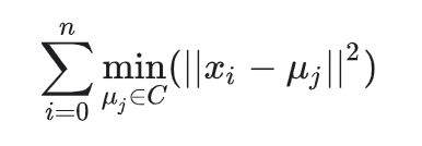
这里n是数据集中的记录数，xi是第i个数据点，C是聚类数，而µj是第j个质心。

使用k均值聚类进行客户细分的一个缺点或困难是，我们需要事先知道聚类的数量。但是，通常我们不知道要创建的最佳群集数是多少。轮廓系数可用于评估并帮助确定针对分割问题的最佳聚类数量。简而言之，轮廓系数衡量的是数据点与其他群集相比与群集之间的距离

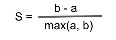
其中b是点与其最接近的簇之间的距离的平均值，而a是同一簇内的数据点之间的平均距离。轮廓系数值的范围是-1至1，其中值越接近1，则效果越好。

在这篇文章里,我会使用一个在线零售的数据集，仍然是来自Kaggle，数据集是OnlineRetail.csv 。我们将使用k-means聚类算法构建客户细分模型。

# This Python 3 environment comes with many helpful analytics libraries installed
# It is defined by the kaggle/python Docker image: https://github.com/kaggle/docker-python
# For example, here's several helpful packages to load

import numpy as np # linear algebra
import pandas as pd # data processing, CSV file I/O (e.g. pd.read_csv)

# Input data files are available in the read-only "../input/" directory
# For example, running this (by clicking run or pressing Shift+Enter) will list all files under the input directory

import os
for dirname, _, filenames in os.walk('/kaggle/input'):
    for filename in filenames:
        print(os.path.join(dirname, filename))

# You can write up to 5GB to the current directory (/kaggle/working/) that gets preserved as output when you create a version using "Save & Run All" 
# You can also write temporary files to /kaggle/temp/, but they won't be saved outside of the current session

/kaggle/input/onlineretail/OnlineRetail.csv

Load packages

import matplotlib.pyplot as plt
import pandas as pd
import numpy as np
from sklearn.cluster import KMeans
from sklearn.metrics import silhouette_score
%matplotlib inline

Load the data

df=pd.read_csv(r"../input/onlineretail/OnlineRetail.csv", encoding="cp1252")
df.head(3)

	InvoiceNo	StockCode	Description	Quantity	InvoiceDate	UnitPrice	CustomerID	Country
0	536365	85123A	WHITE HANGING HEART T-LIGHT HOLDER	6	12/1/2010 8:26	2.55	17850.0	United Kingdom
1	536365	71053	WHITE METAL LANTERN	6	12/1/2010 8:26	3.39	17850.0	United Kingdom
2	536365	84406B	CREAM CUPID HEARTS COAT HANGER	8	12/1/2010 8:26	2.75	17850.0	United Kingdom

Data Cleaning

df = df.loc[df['Quantity'] > 0]  # remove negative Quantity
df = df[pd.notnull(df['CustomerID'])]  # remove missing customer ID
df = df.loc[df['InvoiceDate'] < '2011-12-01'] # remove incomeplete month
df['Sales'] = df['Quantity'] * df['UnitPrice'] # create total sale

customer_df = df.groupby('CustomerID').agg({
    'Sales': sum,
    'InvoiceNo': lambda x: x.nunique()
})

customer_df.columns = ['TotalSales', 'OrderCount']
customer_df['AvgOrderValue'] = customer_df['TotalSales']/customer_df['OrderCount']

rank_df = customer_df.rank(method='first')
normalized_df = (rank_df - rank_df.mean()) / rank_df.std()

Customer Segmentation via K-Means Clustering

kmeans = KMeans(n_clusters=4).fit(normalized_df[['TotalSales', 'OrderCount', 'AvgOrderValue']])

kmeans

KMeans(algorithm='auto', copy_x=True, init='k-means++', max_iter=300,
       n_clusters=4, n_init=10, n_jobs=None, precompute_distances='auto',
       random_state=None, tol=0.0001, verbose=0)

kmeans.labels_

array([3, 2, 2, ..., 0, 1, 2], dtype=int32)

kmeans.cluster_centers_

array([[-1.24238492, -0.72361466, -1.04323974],
       [ 0.22963624,  0.77161017, -0.57743064],
       [ 1.20050352,  0.95015985,  0.93261073],
       [-0.04345453, -0.93680013,  0.81681633]])

four_cluster_df = normalized_df[['TotalSales', 'OrderCount', 'AvgOrderValue']].copy(deep=True)
four_cluster_df['Cluster'] = kmeans.labels_
four_cluster_df

	TotalSales	OrderCount	AvgOrderValue	Cluster
CustomerID
12346.0	1.728056	-1.731252	1.730186	3
12347.0	1.469167	1.038751	1.366890	2
12348.0	0.904512	-0.101212	1.211344	2
12349.0	1.247567	-1.730186	1.676917	3
12350.0	-0.504993	-1.729121	0.365427	3
...	...	...	...	...
18276.0	-0.498601	-0.104408	0.372885	3
18277.0	-1.525632	-0.103342	-1.442532	0
18282.0	-1.638563	-0.102277	-1.601275	0
18283.0	1.044078	1.623648	-1.193232	1
18287.0	0.867224	0.675455	1.161270	2

3251 rows ?? 4 columns

plt.scatter(
    four_cluster_df.loc[four_cluster_df['Cluster'] == 0]['OrderCount'], 
    four_cluster_df.loc[four_cluster_df['Cluster'] == 0]['TotalSales'],
    c='blue'
)

plt.scatter(
    four_cluster_df.loc[four_cluster_df['Cluster'] == 1]['OrderCount'], 
    four_cluster_df.loc[four_cluster_df['Cluster'] == 1]['TotalSales'],
    c='red'
)

plt.scatter(
    four_cluster_df.loc[four_cluster_df['Cluster'] == 2]['OrderCount'], 
    four_cluster_df.loc[four_cluster_df['Cluster'] == 2]['TotalSales'],
    c='orange'
)

plt.scatter(
    four_cluster_df.loc[four_cluster_df['Cluster'] == 3]['OrderCount'], 
    four_cluster_df.loc[four_cluster_df['Cluster'] == 3]['TotalSales'],
    c='green'
)

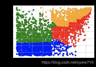
plt.title('TotalSales vs. OrderCount Clusters')
plt.xlabel('Order Count')
plt.ylabel('Total Sales')

plt.grid()
plt.show()


plt.scatter(
    four_cluster_df.loc[four_cluster_df['Cluster'] == 0]['OrderCount'], 
    four_cluster_df.loc[four_cluster_df['Cluster'] == 0]['AvgOrderValue'],
    c='blue'
)

plt.scatter(
    four_cluster_df.loc[four_cluster_df['Cluster'] == 1]['OrderCount'], 
    four_cluster_df.loc[four_cluster_df['Cluster'] == 1]['AvgOrderValue'],
    c='red'
)

plt.scatter(
    four_cluster_df.loc[four_cluster_df['Cluster'] == 2]['OrderCount'], 
    four_cluster_df.loc[four_cluster_df['Cluster'] == 2]['AvgOrderValue'],
    c='orange'
)

plt.scatter(
    four_cluster_df.loc[four_cluster_df['Cluster'] == 3]['OrderCount'], 
    four_cluster_df.loc[four_cluster_df['Cluster'] == 3]['AvgOrderValue'],
    c='green'
)

plt.title('AvgOrderValue vs. OrderCount Clusters')
plt.xlabel('Order Count')
plt.ylabel('Avg Order Value')

plt.grid()
plt.show()


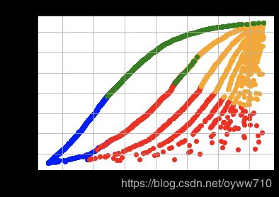
plt.scatter(
    four_cluster_df.loc[four_cluster_df['Cluster'] == 0]['TotalSales'], 
    four_cluster_df.loc[four_cluster_df['Cluster'] == 0]['AvgOrderValue'],
    c='blue'
)

plt.scatter(
    four_cluster_df.loc[four_cluster_df['Cluster'] == 1]['TotalSales'], 
    four_cluster_df.loc[four_cluster_df['Cluster'] == 1]['AvgOrderValue'],
    c='red'
)

plt.scatter(
    four_cluster_df.loc[four_cluster_df['Cluster'] == 2]['TotalSales'], 
    four_cluster_df.loc[four_cluster_df['Cluster'] == 2]['AvgOrderValue'],
    c='orange'
)

plt.scatter(
    four_cluster_df.loc[four_cluster_df['Cluster'] == 3]['TotalSales'], 
    four_cluster_df.loc[four_cluster_df['Cluster'] == 3]['AvgOrderValue'],
    c='green'
)

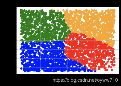
plt.title('AvgOrderValue vs. TotalSales Clusters')
plt.xlabel('Total Sales')
plt.ylabel('Avg Order Value')

plt.grid()
plt.show()

Selecting the best number of clusters

for n_cluster in [4,5,6,7,8]:
    kmeans = KMeans(n_clusters=n_cluster).fit(
        normalized_df[['TotalSales', 'OrderCount', 'AvgOrderValue']]
    )
    silhouette_avg = silhouette_score(
        normalized_df[['TotalSales', 'OrderCount', 'AvgOrderValue']], 
        kmeans.labels_
    )
    
    print('Silhouette Score for %i Clusters: %0.4f' % (n_cluster, silhouette_avg))

Silhouette Score for 4 Clusters: 0.4213
Silhouette Score for 5 Clusters: 0.3823
Silhouette Score for 6 Clusters: 0.3663
Silhouette Score for 7 Clusters: 0.3860
Silhouette Score for 8 Clusters: 0.3650

In our case, of the five different numbers of clusters we have experimented with, the best number of clusters with the highest silhouette score was 4