卷积神经网络结构总结（一）

10.17

常规的神经网络

传统的神经网络并不能很好的适配输入图像的大小，如2002003的图像，在传统的神经网络中使用全连接层，每个神经元需要学习的权重矩阵就有120,000（2002003）个，并且传统网络中还有很多个神经元，所以全连接的方式十分浪费资源并且会很快造成过度拟合（overfitting）。

卷积神经网络

3D体积的神经元，CNN的每一层的神经元在3D尺度上（the layers of a ConvNet have neurons arranged in 3 dimensions: width, height, depth）卷积网络的构建通常包括三种类型的层（layer）：

• 卷积层（Convolutional Layer）
• 池化层（Pooling Layer）
• 全连接层（ Fully-Connected Layer）

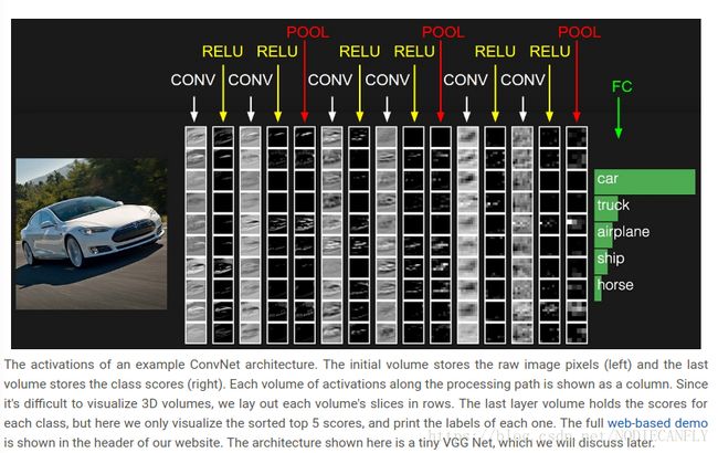
下面我们简单举一个卷及神经网络的例子（a simple ConvNet for CIFAR-10 classification）
architecture：[INPUT - CONV - RELU - POOL - FC]

• INPUT [32323] 输入图像的尺寸大小是32323，最后的3是图像的RGB颜色通道
• CONV ：卷积层如果我们首使用10个5×5×3的卷积核，那么最后得到的结果是28×28×10，关于卷积结果和步长（Stride）的问题我们稍后讲解。
• RELU层：输入[282810]，将使用一种激活函数，例如max(0, x)阈值为0。经过这一层的输出没有变化，还是[282810]
• POOLING 层：输入[282810]，池化层是在空域上对输入的图像进行下采样（width,height）,输出结果为[141410]
• FC(fully-connected)层：这一层将计算分类的得分输出为[1110]，每一个数字对应 CIFAR-10中的一类图片的得分

通过这种方式，卷及神经网络将我们输入的一张图片映射到最后的分类得分。注意一些层 中含有参数（parameters，注意区分参数和超参数），一些层中不含有参数。特别是 CONV/FC 层应用的函数不仅仅是激活该层的输入矩阵，还激活了该层的参数（the weights and biases of the neurons）。相应的， RELU/POOL 层应用的是固定的函数。CONV/FC 中的参数会在训练过程中应用梯度下降的方法不断的调整，使得最后的分类得分与图像原有的标签更加一致。

总结 ：

• 神经网络的结构在上面的例子中就是一系列层的叠加，将输入的图像转化为最后的分类得分
• 现在有许多不同功能的层（上面介绍的四种是最常使用的）
• 每一层接受一个三维的输入，并且通过一定的函数转化为三维的输出
• 每一层可能含有参数（CONV/FC do, RELU/POOL don’t）
• 每一层可能含有超参数（CONV/FC/POOL do, RELU doesn’t）
  

下面我们将详细介绍各层的超参数和连接的细节

卷基层

卷基层是卷积网络的核心，完成大量的计算任务

1.概述

CONV层的参数包含一系列的线性滤波器，每个滤波器的长宽都很小（width and height），但是和输入矩阵具有同样的深度，例如我们上面举的553的滤波器的例子，当它在我们的图像上不断滑动进行卷积运算后得到一个二维的激活图（activation map）表示的是滤波器在每一个空域像素点上的响应。我们将这些activation map按照深度方向排列（深度的大小即滤波器的个数），得到最后的输出三维矩阵。

2.局部连接（Local Connectivity）：

当我们的输入是类似图片的高维输入时，我们看到以全连接的方式连接神经元是不可行的。
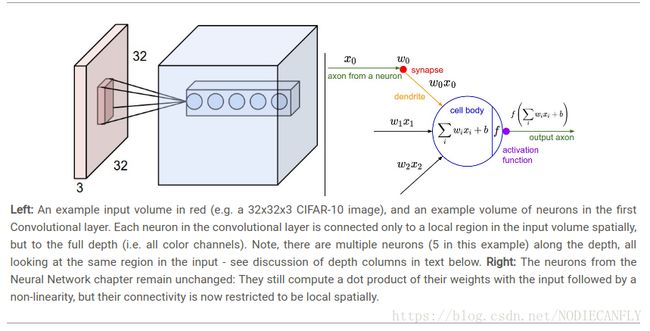
但我们使用卷及网络时，一层中的神经元只能连接到它之前层的一个小区域（感受野），而不是以完全连接的方式连接到所有的神经元。这个连接区域的的大小（就是滤波器的大小）是超参数，成为神经元的感受野（receptive field ）需要再次强调的是这种连接的局部性针对的是空域（width and height）但是在深度上和输入图像是一样的。

Example 1. For example, suppose that the input volume has size [32x32x3], (e.g. an RGB CIFAR-10 image). If the receptive field (or the filter size) is 5x5, then each neuron in the Conv Layer will have weights to a [5x5x3] region in the input volume, for a total of 553 = 75 weights (and +1 bias parameter). Notice that the extent of the connectivity along the depth axis must be 3, since this is the depth of the input volume.
Example 2. Suppose an input volume had size [16x16x20]. Then using an example receptive field size of 3x3, every neuron in the Conv Layer would now have a total of 3320 = 180 connections to the input volume. Notice that, again, the connectivity is local in space (e.g. 3x3), but full along the input depth (20).

这里讲解一下上图：中间蓝色正方体中每5个球代表的是5个不同553神经元卷积得到的结果

3. 空间排列

下面是怎样计算输出矩阵的问题（size of out put volumn）:depth, stride, zero-padding

1. 首先是输出矩阵的深度depth ，矩阵的深度是超参数，它等于我们使用的滤波器个数，每一个滤波器都学习在我们的输入图像中去寻找不同的特征。 例如，在第一层神经元我们输入的是原始图像，然后，沿着深度维度的不同神经元可以在存在各种定向边缘或颜色斑点的情况下激活。 这些不同的神经元排列起来形成深度depth.
2. 其次我们要确定我们在滑动滤波器时的步长stride ，例如步长为1时，我们的滤波器每次移动1个像素
3. zero-padding ，有时候在输入图像的边缘进行零填充是很方便的。零填充的尺寸是超参数。zero-padding的好处是允许我们控制输出矩阵的尺寸，例如上图中32×32×3的图像当我们用553的滤波器进行，如果不进行零填充的话，输出矩阵为2828，但是我们可以通过零填充使得我们的输出矩阵和输入保持同样的尺寸3232。这也是zero-padding最常见的用法。

下面是详细的输出矩阵尺寸的计算：

We can compute the spatial size of the output volume as a function of the input volume size (W), the receptive field size of the Conv Layer neurons (F), the stride with which they are applied (S), and the amount of zero padding used § on the border. You can convince yourself that the correct formula for calculating how many neurons “fit” is given by (W−F+2P)/S+1 . For example for a 7x7 input and a 3x3 filter with stride 1 and pad 0 we would get a 5x5 output. With stride 2 we would get a 3x3 output.

In general, setting zero padding to be P=(F−1)/2 when the stride is S=1 ensures that the input volume and output volume will have the same size spatially.

步长的约束：防止我们的输出层非整数

Constraints on strides. Note again that the spatial arrangement hyperparameters have mutual constraints. For example, when the input has size W=10, no zero-padding is used P=0, and the filter size is F=3, then it would be impossible to use stride S=2, since (W−F+2P)/S+1=(10−3+0)/2+1=4.5, i.e. not an integer, indicating that the neurons don’t “fit” neatly and symmetrically across the input. Therefore, this setting of the hyperparameters is considered to be invalid, and a ConvNet library could throw an exception or zero pad the rest to make it fit, or crop the input to make it fit, or something. As we will see in the ConvNet architectures section, sizing the ConvNets appropriately so that all the dimensions “work out” can be a real headache, which the use of zero-padding and some design guidelines will significantly alleviate.

现实中的卷积神经网络举例：

Real-world example. The Krizhevsky et al. architecture that won the ImageNet challenge in 2012 accepted images of size [227x227x3]. On the first Convolutional Layer, it used neurons with receptive field size F=11, stride S=4 and no zero padding P=0. Since (227 - 11)/4 + 1 = 55, and since the Conv layer had a depth of K=96, the Conv layer output volume had size [55x55x96]. Each of the 555596 neurons in this volume was connected to a region of size [11x11x3] in the input volume. Moreover, all 96 neurons in each depth column are connected to the same [11x11x3] region of the input, but of course with different weights. As a fun aside, if you read the actual paper it claims that the input images were 224x224, which is surely incorrect because (224 - 11)/4 + 1 is quite clearly not an integer. This has confused many people in the history of ConvNets and little is known about what happened. My own best guess is that Alex used zero-padding of 3 extra pixels that he does not mention in the paper.

真实世界的例子。 Krizhevsky等赢得2012年ImageNet挑战的架构接受了大小[227x227x3]的图像。在第一个卷积层上，它使用感野大小为F = 11的神经元，步长S = 4，零填充P = 0。由于（227-11）/ 4 + 1 = 55，并且由于Conv层具有K = 96的深度，所以Conv层输出体积具有尺寸[55×55×96]。volume中的每个55 * 55 * 96神经元连接到输入体积大小为[11x11x3]的区域。此外，每个深度列中的所有96个神经元连接到输入的相同的[11x11x3]区域，但是当然具有不同的权重。除此之外，如果你读到实际的论文，它声称输入图像是224×224，这肯定是不正确的，因为（224 - 11）/ 4 + 1很明显不是一个整数。这让ConvNets的历史上很多人感到困惑，对发生的事情知之甚少。我自己最好的猜测是，Alex使用了他在本文中没有提到的3个额外像素的零填充。

4. 参数共享（Parameter Sharing）

Parameter sharing策略是在卷积神经网络中使用的控制参数规模的方法。在上面的例子中，我们看到在第一个卷积层有 555596 = 290,400个神经元，每一个神经元有11×11×3=363 个权重参数和1个偏差（bias），总的加起来有 290,400×363 = 105,705,600 个参数，仅仅在第一个卷积层。很明显，参数的个数太多了。
所以我们可以做出一个合理的假设来明显减少参数的个数：如果一个特征对于在某个空间位置（x，y）计算是有用的，那么在不同的位置（x2 ，y2）上。换句话说，将一个二维深度切片表示为一个深度切片（例如，大小为[55x55x96]的volume具有96个深度切片，每个切片的大小为[55x55]），我们将限制每个深度切片中的神经元使用相同的权重和偏见。使用这个参数共享方案，我们例子中的第一个Conv层现在将只有96个独特权重集（每个深度切片一个权重集），总共96 * 11 * 11 * 3 = 34,848个唯一权重或34,944个参数+96偏见）。或者，每个深度切片中的所有55 * 55个神经元现在将使用相同的参数。在反向传播的实践中，volume中的每个神经元将计算其权重的梯度，但这些梯度将叠加在每个深度切片上，并且仅更新每个切片的一组权重。
简单的理解就是我们使用一个滤波模板对整幅进行卷积操作。这一组权重称之为filter（kernel）

---

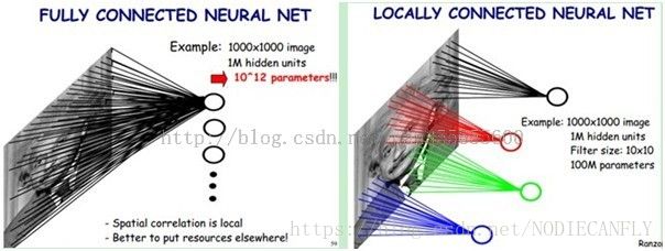
通过感受野和参数共享减少训练网络训练的参数个数，下面是一个具体的例子：若我们有1000x1000像素的图像，有1百万个隐藏层的神经元，如果全连接（即每个隐层神经元都要与图像的每一个像素点进行连接），就有1000x1000x1000000=10^ 12个连接，也就是10^12个权值参数。但是图像的空间联系是局部的，就像人是通过一个局部的感受野去感受外界图像一样，每一个神经元都不需要对全局图像做感受，因为每个神经元只感受局部的图像区域，然后在更高层，将这些感受不同局部的神经元综合起来可得到全局信息。这样，我们就可以减少连接的数目，即减少神经网络需要训练的权值参数的个数了。来自Depatime的博客。

如有图所示：假如局部感受野是10x10，则隐层每个感受野只需要和这10x10的局部图像相连接，所以1百万个隐层神经元就只有一亿个连接，即10^8个参数。这样训练起来就没那么费力了，但还是感觉有点多，有其它方法吗？
我们知道，隐藏层的每一个神经元都连接10x10个元素的图像区域，也就是说每一个神经元存在10x10=100个连接权值参数。如果我们每个神经元这100个参数是相同的呢？也就是说每个神经元用的是同一个卷积核去卷积图像。这样我们就只有多少个参数呢？？只有100个参数（从10的8次方到10的2次方）天壤之别！！！不管你隐层的神经元个数有多少，两层间的连接就只有100个参数啊，这就是权值共享啊！即卷积神经网络的亮点之一。
一种滤波器，也就是一种卷积核就是提取出图像的一种特征，例如某个方向的边缘。那么我们需要提取不同的特征，则可以怎么办，加多几种滤波器不就行了吗？所以假设我们加到50，每种滤波器的参数不一样，表示它提出输入图像的不同特征，例如不同的边缘。这样每种滤波器去卷积图像就得到对图像的不同特征的放映，我们称之为Feature Map。所以50种卷积核就有对应的50个Feature Map。这50个Feature Map就组成了一层神经元。我们这一层有多少个参数了？50种卷积核x每种卷积核共享100个参数=50*100，也就是5000个参数，达到了我们想要 的效果，不仅可以提取多方面的特征而且还可以减少计算。见上图右：不同的颜色表示不同的滤波器。

---

需要注意的是：图片的特征可以分为底层特征和高级特征。图像的底层特征与特征在图像中的位置无关 ，比如说边缘，无论边缘在图像的中心还是四周，我们都可以用边缘检测算子进行滤波操作检验出来。但是高级特征一般与位置有关， 比如一张人脸，眼睛和嘴的位置不同，那么处理到高层，不同的位置就要用不同的权重，这时候卷积层就不能胜任了，需要用局部连接层或者全连接层。
举例：
假设我们的输入为X

• A depth column (or a fibre) at position (x,y) would be the activations X[x,y,:].
• A depth slice, or equivalently an activation map at depth d would be the activations X[:,:,d].

卷积层举例：
Suppose that the input volume X has shape X.shape: (11,11,4). Suppose further that we use no zero padding (P=0), that the filter size is F=5, and that the stride is S=2. The output volume would therefore have spatial size (11-5)/2+1 = 4, giving a volume with width and height of 4. The activation map in the output volume (call it V), would then look as follows (only some of the elements are computed in this example):

• V[0,0,0] = np.sum(X[:5,:5,:] * W0) + b0
• V[1,0,0] = np.sum(X[2:7,:5,:] * W0) + b0
• V[2,0,0] = np.sum(X[4:9,:5,:] * W0) + b0
• V[3,0,0] = np.sum(X[6:11,:5,:] * W0) + b0

Remember that in numpy, the operation * above denotes elementwise multiplication between the arrays. Notice also that the weight vector W0 is the weight vector of that neuron and b0 is the bias. Here, W0 is assumed to be of shape W0.shape: (5,5,4), since the filter size is 5 and the depth of the input volume is 4. Notice that at each point, we are computing the dot product as seen before in ordinary neural networks. Also, we see that we are using the same weight and bias (due to parameter sharing), and where the dimensions along the width are increasing in steps of 2 (i.e. the stride). To construct a second activation map in the output volume, we would have:

V[0,0,1] = np.sum(X[:5,:5,:] * W1) + b1
V[1,0,1] = np.sum(X[2:7,:5,:] * W1) + b1
V[2,0,1] = np.sum(X[4:9,:5,:] * W1) + b1
V[3,0,1] = np.sum(X[6:11,:5,:] * W1) + b1
V[0,1,1] = np.sum(X[:5,2:7,:] * W1) + b1 (example of going along y)
V[2,3,1] = np.sum(X[4:9,6:11,:] * W1) + b1 (or along both)

where we see that we are indexing into the second depth dimension in V (at index 1) because we are computing the second activation map, and that a different set of parameters (W1) is now used. In the example above, we are for brevity leaving out some of the other operations the Conv Layer would perform to fill the other parts of the output array V. Additionally, recall that these activation maps are often followed elementwise through an activation function such as ReLU, but this is not shown here.

Summary . To summarize, the Conv Layer:

• Accepts a volume of size W1×H1×D1
• Requires four hyperparameters:
  - Number of filters K,
  - their spatial extent F,
  - the stride S,
  - the amount of zero padding P.
• Produces a volume of size W2×H2×D2 where:
  - W2=(W1−F+2P)/S+1
  - H2=(H1−F+2P)/S+1 (i.e. width and height are computed equally by symmetry)
  - D2=K
• With parameter sharing, it introduces F⋅F⋅D1 weights per filter, for a total of (F⋅F⋅D1)⋅K weights and K biases.
• In the output volume, the d-th depth slice (of size W2×H2) is the result of performing a valid convolution of the d-th filter over the input volume with a stride of S, and then offset by d-th bias.

A common setting of the hyperparameters is F=3,S=1,P=1. However, there are common conventions and rules of thumb that motivate these hyperparameters. See the ConvNet architectures section below.

Implementation as Matrix Multiplication 矩阵实现卷积

1. The local regions in the input image are stretched out into columns in an operation commonly called im2col. For example, if the input is [227x227x3] and it is to be convolved with 11x11x3 filters at stride 4, then we would take [11x11x3] blocks of pixels in the input and stretch each block into a column vector of size 11113 = 363. Iterating this process in the input at stride of 4 gives (227-11)/4+1 = 55 locations along both width and height, leading to an output matrix X_col of im2col of size [363 x 3025], where every column is a stretched out receptive field and there are 55*55 = 3025 of them in total. Note that since the receptive fields overlap, every number in the input volume may be duplicated in multiple distinct columns.
2. The weights of the CONV layer are similarly stretched out into rows. For example, if there are 96 filters of size [11x11x3] this would give a matrix W_row of size [96 x 363].
3. The result of a convolution is now equivalent to performing one large matrix multiply np.dot(W_row, X_col), which evaluates the dot product between every filter and every receptive field location. In our example, the output of this operation would be [96 x 3025], giving the output of the dot product of each filter at each location.
4. The result must finally be reshaped back to its proper output dimension [55x55x96].

This approach has the downside that it can use a lot of memory, since some values in the input volume are replicated multiple times in X_col. However, the benefit is that there are many very efficient implementations of Matrix Multiplication that we can take advantage of. Moreover, the same im2col idea can be reused to perform the pooling operation, which we discuss next.
这里用矩阵乘法可以提高运算效率，降低时间复杂度
参考cs231 convolutional-networks http://cs231n.github.io/convolutional-networks/

池化层

周期性地在ConvNet体系结构中连续的Conv层之间插入一个Pooling层。 其功能是逐步减小表示的空间大小，以减少网络中的参数和计算量，从而也控制过拟合。 池层在输入的每个深度切片上独立运行，并使用MAX操作在空间上调整其大小。 最常见的形式是一个大小为2x2的过滤器的汇聚层，在输入的每个深度切片上沿着宽度和高度两次施加2个下采样的步幅，丢弃75％的激活。 在这种情况下，每个MAX操作最多需要超过4个数字（在某个深度切片中，只有很少的2×2区域）。 深度维度保持不变。 更一般地说，池化层：

• Accepts a volume of size W1×H1×D1输入volume的大小
• Requires two hyperparameters: their spatial extent F,the stride S两个超参数，填充F，步长S
• Produces a volume of size W2×H2×D2 where:输出volume大小
• W2=(W1−F)/S+1
  H2=(H1−F)/S+1
  D2=D1
• Introduces zero parameters since it computes a fixed function of the input
• For Pooling layers, it is not common to pad the input using zero-padding.

It is worth noting that there are only two commonly seen variations of the max pooling layer found in practice: A pooling layer with F=3,S=2 (also called overlapping pooling), and more commonly F=2,S=2. Pooling sizes with larger receptive fields are too destructive.
General pooling. :In addition to max pooling, the pooling units can also perform other functions, such as average pooling or even L2-norm pooling. Average pooling was often used historically but has recently fallen out of favor compared to the max pooling operation, which has been shown to work better in practice.
通常池化，是最大池化，平均数池化，L2-norm池化。历史上使用平均池化最多。但最近大家都是使用最大池化，效果比较好。

Backpropagation. Recall from the backpropagation chapter that the backward pass for a max(x, y) operation has a simple interpretation as only routing the gradient to the input that had the highest value in the forward pass. Hence, during the forward pass of a pooling layer it is common to keep track of the index of the max activation (sometimes also called the switches) so that gradient routing is efficient during backpropagation.
回顾一下反向传播算法，因为池化追求的是最大值，保证的梯度的有效性。

Getting rid of pooling . Many people dislike the pooling operation and think that we can get away without it. For example, Striving for Simplicity: The All Convolutional Net proposes to discard the pooling layer in favor of architecture that only consists of repeated CONV layers. To reduce the size of the representation they suggest using larger stride in CONV layer once in a while. Discarding pooling layers has also been found to be important in training good generative models, such as variational autoencoders (VAEs) or generative adversarial networks (GANs). It seems likely that future architectures will feature very few to no pooling layers.
抛弃池化层，很多人不喜欢池化操作，并且认为应该抛弃。例如：争取模型简单，卷积网络中，只存在重复的卷积操作，我们使用比较大的步长减少参数。抛弃池化层，已经被证实在（变分自动编码器）VAEs,（生成对抗网络）GANs中，并取得不错的效果。似乎未来不需要池化操作。

Normalization Layer

Many types of normalization layers have been proposed for use in ConvNet architectures, sometimes with the intentions of implementing inhibition schemes observed in the biological brain. However, these layers have since fallen out of favor because in practice their contribution has been shown to be minimal, if any. For various types of normalizations, see the discussion in Alex Krizhevsky’s cuda-convnet library API.
许多类型归一化层被应用到ConvNet结构中，这种倾向是来源于观察生物大脑给出的inhibition schemes。然而，这种归一化操作已经失宠，因为在实际操作中，它所带来的作用是非常小的。更多归一化操作，请看Alex Krizhevsky的cuda-convnet 的API.

Fully-connected layer

Neurons in a fully connected layer have full connections to all activations in the previous layer, as seen in regular Neural Networks. Their activations can hence be computed with a matrix multiplication followed by a bias offset. See the Neural Network section of the notes for more information.
完整连接层中的神经元与前一层中的所有激活都有完全连接，正如在常规神经网络中所见。 因此可以用一个矩阵乘法和一个偏置偏移来计算它们的激活。 有关更多信息，请参阅笔记的“神经网络”部分。

Converting FC layers to CONV layers

It is worth noting that the only difference between FC and CONV layers is that the neurons in the CONV layer are connected only to a local region in the input, and that many of the neurons in a CONV volume share parameters. However, the neurons in both layers still compute dot products, so their functional form is identical. Therefore, it turns out that it’s possible to convert between FC and CONV layers:

值得注意的是，FC和CONV层之间的唯一区别在于，CONV层中的神经元仅连接到输入中的局部区域，并且CONV中的许多神经元共享参数。 然而，两层神经元仍然计算点积，所以它们的功能形式是相同的。 因此，可以在FC和CONV层之间进行转换

• For any CONV layer there is an FC layer that implements the same forward function. The weight matrix would be a large matrix that is mostly zero except for at certain blocks (due to local connectivity) where the weights in many of the blocks are equal (due to parameter sharing).
• Conversely, any FC layer can be converted to a CONV layer. For example, an FC layer with K=4096 that is looking at some input volume of size 7×7×512 can be equivalently expressed as a CONV layer with F=7,P=0,S=1,K=4096. In other words, we are setting the filter size to be exactly the size of the input volume, and hence the output will simply be 1×1×4096 since only a single depth column “fits” across the input volume, giving identical result as the initial FC layer.

FC->CONV conversion . Of these two conversions, the ability to convert an FC layer to a CONV layer is particularly useful in practice. Consider a ConvNet architecture that takes a 224x224x3 image, and then uses a series of CONV layers and POOL layers to reduce the image to an activations volume of size 7x7x512 (in an AlexNet architecture that we’ll see later, this is done by use of 5 pooling layers that downsample the input spatially by a factor of two each time, making the final spatial size 224/2/2/2/2/2 = 7). From there, an AlexNet uses two FC layers of size 4096 and finally the last FC layers with 1000 neurons that compute the class scores. We can convert each of these three FC layers to CONV layers as described above:
FC-> CONV转换。 在这两种转换中，将FC层转换为CONV层的能力在实践中特别有用。 考虑一个采用224x224x3图像的ConvNet体系结构，然后使用一系列CONV图层和POOL图层将图像缩小为7x7x512的激活volume（在AlexNet体系结构中，我们稍后会看到，这是通过使用 5个池化层，每次对输入进行空间下采样，使得最终的空间尺寸为224/2/2/2/2/2 = 7）。 从那里，一个AlexNet使用两个大小为4096的FC层，最后使用1000个神经元计算类分数。 我们可以将这三个FC层中的每一个转换为CONV层，如上所述