通过代码学习 VQ-VAE

VQ-VAE（Vector Quantised Variational AutoEncoder，矢量量化变分自动编码）是【1】提出的一种离散化VAE方案，近来【2】应用VQ-VAE得到了媲美于BigGan的生成模型。由此可见， VQ-VAE 有着强大的潜力，且【1】和【2】皆为DeepMind的作品，让我们通过代码来认识它，学习它。

一、简介

光看论文一知半解，需要看看它的实现。我在GitHub中找到一个很简单的代码【3】，不妨一起研究研究。以下叙述是结合【3】的实现一起叙述的。
VQ-VAE属于VAE范畴，它有着与一般VAE都有的Encoder、code（编码）和Decoder，而不同之处在于其code并不是由Encoder直接输出得到，而是经过了一个矢量量化后才得到的，其结构图如下：

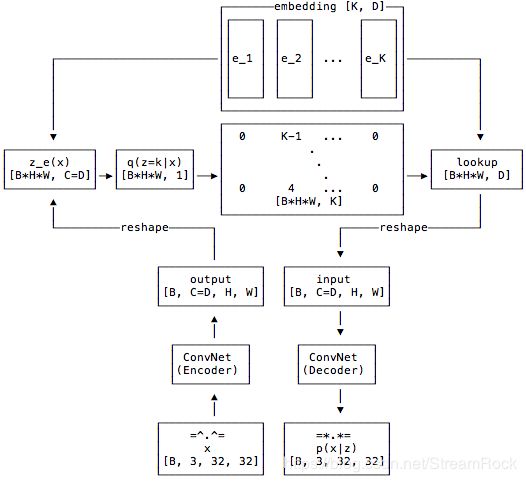
图1 VQ-VAE结构图【3】

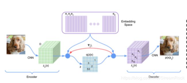
图2 VQ-VAE数据流图【1】

结合 图1、图2 叙述其工作流程

1. 输入x，其数据结构为[B,3,32,32]，由于【3】采用了CIFAR10作为训练集，因此输入参数如此，B是batch的数量；
2. 经过Encoder，得到 $Z_e(x)$, 其结构为 [B, C=D, H, W]，其中C是指编码器的Conv网络输出的Channels 的数量，而D是指矢量量化中矢量的维度，也就是后续查表（Embedding）所存储矢量的维度，另外，H,W表示输入图像经编码器处理后的长和宽，本例中，编码器输入是32 * 32，输出时为8 * 8，即H=8, W=8；
3. 将 $Z_e(x)$ 变形为 [B * H * W, D]，即每一个图片有 H*W 个编码，每个编码是D维，计算这些编码（B * H * W）与 Embedding 中 K 个矢量（在【3】中 K=512，表示矢量量化编码的矢量个数)之间的距离，通过最近邻算法构成如下映射：
   $$q(z=k|x)=\{\begin{array}{cc}1& \text{for }k=\arg {\min }_j\Vert Z_e(x)-e_j{\Vert }_2\\ 0& \text{otherwise}\end{array}(1)$$
   公式（1）表示当输入为 $x$ 时，$z=k$ 的概率是 ：1）当 $k$ 是矢量序列 $\{e_1,e_2,\cdots ,e_K\}$中与 $Z_e(x)$ 最近的矢量的下标时，条件概率为1；2）否则为0。这里的矢量距离度量采用常见的欧拉距离 $\Vert \cdot {\Vert }_2$，公式（1）便是最近邻算法的实现。
   $$z_q(x)=e_k\text{where}k=\arg \underset{j}{\min }\Vert Z_e(x)-e_j{\Vert }_2(2)$$
   公式（2）表示的是，通过最近邻计算出与 $Z_e(x)$ 最近的矢量的下标为 $k$，然后查表将 $e_k$ 输出作为编码输出 $z_q(x)$。
4. $z_q(x)$ 作为Decoder的输入，有Decoder重建图像，输出 $p(x|z)$。

由上分析，我们得知VQ-VAE的输出的每一个编码都是离散的，它们是保存在 Embedding 中 K个矢量中的某一个。在[3]的实验中，一幅图片在矢量量化后，将由8 * 8 个 64 维矢量表示，而这里的每个矢量都是 Embedding 中512个矢量中的一个。
在整个实现中，有两个部分是很有特点的，其一就是上面讲的矢量量化过程，另外一个就是Loss的计算。在[1]中，Loss分为三个部分，如下：
$$Loss=\log p(x|z_q(x))+\Vert sg[Z_e(x)]-e{\Vert }_2^2+\beta \Vert Z_e(x)-sg[e]{\Vert }_2^2(3)$$
第一项 $\log p(x|z_q(x))$ 表示重构误差，这是二进制交叉熵的形式；第二项是用于update 在 Embedding中的字典项的Loss，其中 $sg[\cdot ]$ 表示 stop gradient，即不执行后向梯度传递，因此，该项只对字典项（矢量量化中矢量）学习有效；第三项是对Encoder有效的Loss，其解释如下：
“Finally, since the volume of the embedding space is dimensionless, it can grow arbitrarily if the embeddings $e_i$ do not train as fast as the encoder parameters. To make sure the encoder commits to an embedding and its output does not grow, we add a commitment loss”
直接翻译过来是：
由于 the embedding space 中的量是无量纲的，如果 $e_i$ 的训练速度跟不上encoder参数的训练速度的话，它就可能增大到任意值。因此，为使encoder能给出一个合理的embedding，于是就给encoder加上了一个惩罚项，其中 $\beta$ 可选为 $[0.1,2]$，本例中选为$\beta =0.25$。
我的理解是，如果encoder与embedding之间若无一个约束的话，则encoder的输出会严重偏离embedding中的矢量，因为前文已经说明了the volume of the embedding space is dimensionless。
另外，在backward时，重构误差梯度信息是直接传给Encoder的，但实际上Encoder的信息并不是直接被Decoder使用的，中间有Embedding转换一道，这是合理的吗？文章【1】给出的解释如下：
During forward computation the nearest embedding $z_q(x)$ (equation 2) is passed to the decoder, and during the backwards pass the gradient ${\nabla }_{z}L$ is passed unaltered to the encoder. Since the output representation of the encoder and the input to the decoder share the same D dimensional space, the gradients contain useful information for how the encoder has to change its output to lower the reconstruction loss.
这就是图2中红线标注出来的地方（${\nabla }_{z}L$），因为Embedding最终输出的矢量维度与Encoder输出矢量的维度相同，而且相似，因此可认为梯度 ${\nabla }_{z}L$ 也可以改善Encoder的重构误差。这种说法虽然不严谨，但从实验结果上看，是行得通的。
小结一下Loss的作用对象：
1、Encoder 受 $\log p(x|z_q(x))$ 和 $\beta \Vert Z_e(x)-sg[e]{\Vert }_2^2$ 影响；
2、Embedding 受 $\log p(x|z_q(x))$ 和 $\Vert sg[Z_e(x)]-e{\Vert }_2^2$ 影响；
3、Decoder 受 $\log p(x|z_q(x))$ 影响。

二、代码实现

完整的代码在[3]中，我们在这里就不一一详述了，只对一些有点特点的部分写一些注释。
我们先来看看 Embedding的实现：

class VectorQuantizer(nn.Module):
    def __init__(self, num_embeddings, embedding_dim, commitment_cost):
        super(VectorQuantizer, self).__init__()
        
        self._embedding_dim = embedding_dim
        self._num_embeddings = num_embeddings
        
        self._embedding = nn.Embedding(self._num_embeddings, self._embedding_dim)
        self._embedding.weight.data.uniform_(-1/self._num_embeddings, 1/self._num_embeddings)
        self._commitment_cost = commitment_cost

    def forward(self, inputs):
        # convert inputs from BCHW -> BHWC
        inputs = inputs.permute(0, 2, 3, 1).contiguous()
        input_shape = inputs.shape
        
        # Flatten input
        flat_input = inputs.view(-1, self._embedding_dim)
        
        # Calculate distances
        distances = (torch.sum(flat_input**2, dim=1, keepdim=True) 
                    + torch.sum(self._embedding.weight**2, dim=1)
                    - 2 * torch.matmul(flat_input, self._embedding.weight.t()))
            
        # Encoding
        encoding_indices = torch.argmin(distances, dim=1).unsqueeze(1)
        encodings = torch.zeros(encoding_indices.shape[0], self._num_embeddings).to(device)
        encodings.scatter_(1, encoding_indices, 1)
        
        # Quantize and unflatten
        quantized = torch.matmul(encodings, self._embedding.weight).view(input_shape)
        
        # Loss
        e_latent_loss = torch.mean((quantized.detach() - inputs)**2)
        q_latent_loss = torch.mean((quantized - inputs.detach())**2)
        loss = q_latent_loss + self._commitment_cost * e_latent_loss
        
        quantized = inputs + (quantized - inputs).detach()
        avg_probs = torch.mean(encodings, dim=0)
        perplexity = torch.exp(-torch.sum(avg_probs * torch.log(avg_probs + 1e-10)))
        
        # convert quantized from BHWC -> BCHW
        return loss, quantized.permute(0, 3, 1, 2).contiguous(), perplexity, encodings

以下将就上述代码进行解读：
1、此处，Embedding通过 nn.Embedding 来实现，其中有 num_embeddings=512，embedding_dim = 64。对它的初始化，仅仅是通过uniform随机分布来设置初值。
2、Encoder的输出是[ B * C * H * W ]，意味着一幅图片经 Encoder 提取的特征值是 [ C * H * W ]，将其整型为 [ H * W， C ] 即一幅图片有 H * W 个特征，每个特征的编码是 C 维。
3、计算距离：

distances = (torch.sum(flat_input**2, dim=1, keepdim=True) 
                    + torch.sum(self._embedding.weight**2, dim=1)
                    - 2 * torch.matmul(flat_input, self._embedding.weight.t()))

其实 torch.sum(flat_input2, dim=1, keepdim=True) 的维度与 torch.sum(self._embedding.weight2, dim=1) 的维度是不同的，前者是2048 * 1，而后者是 512*1，这样加的结果是 2048 * 512，即前者的每一个元素与后者的每一个元素相加得到的结果，得到一个2048 * 512矩阵，恰好与后面的 torch.matmul(flat_input, self._embedding.weight.t()) 维度相同。这里计算的是：
$$\Vert Z_e(x)-e_j{\Vert }_2$$
接下来

# Encoding
        encoding_indices = torch.argmin(distances, dim=1).unsqueeze(1)
        encodings = torch.zeros(encoding_indices.shape[0], self._num_embeddings).to(device)
        encodings.scatter_(1, encoding_indices, 1)

这里是计算
$$k=\arg \underset{j}{\min }\Vert Z_e(x)-e_j{\Vert }_2$$
由torch.argmin(distances, dim=1)获得每一个特征矢量对应的embedding矢量的索引值 k，再由它作为encoding_indices 将 1 分配到形如：[ B * H * W, K] 的矩阵上，其中 K 是embedding 字典中矢量的个数（即 num_embeddings） 。此 k 的形式（即 encodings 的形式）如下：
$$q(z|x)=\left[\begin{array}{ccccc}0& 0& 1& \cdots & 0\\ 0& 1& 0& \cdots & 0\\ ⋮& ⋮& ⋮& \ddots & ⋮\\ 0& 1& 0& \cdots & 0\end{array}\right]$$
EncodingIndices 矩阵共 B * H * W 行，每行有一个 1 其余皆为0， 矩阵共有 K 列，同1列上可以有多个1。
得到EncodingIndices 矩阵后，只需与Embedding矩阵相乘，便可以实现矢量量化的输出，如下：
quantized = torch.matmul(encodings, self._embedding.weight).view(input_shape)
矩阵乘法 [B * H * W, K] * [ K, D] = [ B * H * W, D]，即：
$$\begin{gathered} z_q(x)=\left[\begin{array}{ccccc}0& 0& 1& \cdots & 0\\ 0& 1& 0& \cdots & 0\\ ⋮& ⋮& ⋮& \ddots & ⋮\\ 0& 1& 0& \cdots & 0\end{array}\right]\ast [e_1{e}_2\cdots e_K{]}^T \\ =\left[\begin{array}{c}{e}_3\\ e_2\\ ⋮\\ e_2\end{array}\right] \end{gathered}$$
接下来是计算与 Embedding 相关的 Loss 计算：

 # Loss
        e_latent_loss = torch.mean((quantized.detach() - inputs)**2)
        q_latent_loss = torch.mean((quantized - inputs.detach())**2)
        loss = q_latent_loss + self._commitment_cost * e_latent_loss

这部分代码对应：
$$\Vert sg[Z_e(x)]-e{\Vert }_2^2+\beta \Vert Z_e(x)-sg[e]{\Vert }_2^2$$
上式的 $sg[\cdot ]$ 表示停止梯度（stop gradient），在实现时，我们看到用了Tensor.detach() 来实现，语法理解真是很精准，实现得很简练，这是佩服作者对Pytorch掌握的熟练，什么时候我才能也达到这个高度呢？

至于其他部分的代码，还有值得学习的，但我在这里就不多说了，有兴趣的同学可以看看[3]，原滋原味。

小结：

VQ-VAE 通过离散的矢量对code进行量化和编码，压缩了编码空间，却达到可以媲美连续编码空间的重构效果，为图像的矢量化提供了一种可能的方法。

---

[1] Neural Discrete Representation Learning, arXiv:1711.00937v2 [cs.LG] 30 May 2018
[2] Generating Diverse High-Fidelity Images with VQ-VAE-2，arXiv:1906.00446v1 [cs.LG] 2 Jun 2019
[3] https://github.com/zalandoresearch/pytorch-vq-vae