多目标遗传算法NSGA-Ⅱ与其Python实现多目标投资组合优化问题

对于单目标优化问题，一般的遗传算法可以较为简单的得到较好的结果。但是，当问题扩展到多目标时，原先的遗传算法便不再适用了。因为目标之间通常有着较深的相互关系，一个目标的优化通常会影响到其余的目标，很难能够得到所有目标都达到最优的解。这时候，如何寻找合适的适应度函数便成解决多目标遗传算法的关键。如今，相关的算法已经有很多种了。包括妥协算法（compromise approach），GWASF-GA，SPEA2，NSGA-Ⅱ。其中NSGA-Ⅱ的使用非常广泛。

NSGA-Ⅱ

NSGA-Ⅱ的优点

1.NSGA-Ⅱ提出了快速的非支配(non-dominated)排序，很好的降低了算法的复杂度。一般的多目标算法复杂度为$O(M{N}^3)$，而NSGA-Ⅱ可以做到$O(M{N}^2)$
2.NSGA-Ⅱ改进了原先NSGA算法为保留解多样性而采用的共享函数。提出了拥挤比较算子（crowded-comparison operator)，从而避免了人为输入参数的不确定性。

快速非支配排序

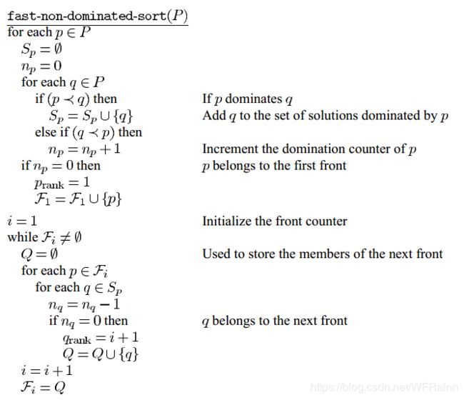
快速非支配排序的核心思想主要是通过计算比较得到种群中每个个体p的被支配度$N_p$,通过支配度的大小得到多层非支配曲面。具体来说过程如下：
对于种群中的每一个个体p，我们计算两个实体。第一个是其被支配度$N_p$，即P个体被其余个体所支配的数量。支配的定义为如果个体p中所有目标均不优于个体q中对应目标，则称个体p被个体q所支配。第二个实体是个体p的支配集合$S_p$。这一步所需要的计算复杂度为$O(M{N}^2)$,因为最坏的情况下，数目为N的种群中每一个个体都要与其余个体比较，这一步为$N^2$，那么对于$M$个目标则为$M{N}^2$。
接下来可以开始寻找非支配曲面了。对于最优非支配曲面(Pareto-optimal front)，其中的个体$N_p$为0。接着，对于最优非支配曲面中的每一个个体，寻找其相应的$S_p$，对于其中所有的个体q，将其$N_p$减1。对于此时$N_p$为0的个体，我们将其归入集合Q，Q便是第二非支配曲面。按照相同的步骤，我们可以得到所有的非支配曲面。由于对于所有个体p，其$N_p$最大为N-1，因此，考虑最坏的情况，即最大$N_p$为N-1，其非支配曲面的个数为N，则为了得到N个曲面所需要的最大遍历的次数为$N^2$。这样，对于M个目标，其计算复杂度为$O(M{N}^2)$。快速非支配排序用算法表达如下：

拥挤比较算子

一般来说，在寻求多目标遗传算法的解时，我们希望解集合能够保存多样性。在NSGA-Ⅱ中，通过运用拥挤比较算子来实现此目的。简单来说，拥挤比较算子的原理如下：
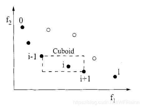
首先定义密度衡量准则（density estimation metric），密度衡量准则定义为一个个体在其每个目标上上下相邻两点的距离。即某个个体与其附近的个体相距越远，密度越小。定义拥挤距离$i_{distance}$定量计算每个个体的密度。拥挤距离的计算需要首先对同一条非支配曲面中每个个体在每个目标上进行升序排序，其中最大值与最小值的个体在此目标上的拥挤距离设为无穷。个体$i$的拥挤距离即等于它在每个目标上$i-1$与$i+1$个体的函数值之差的绝对值之和。在计算时需要标准化每一个目标。两目标的密度表示图如下：

拥挤距离的计算用算法流程表示如下：

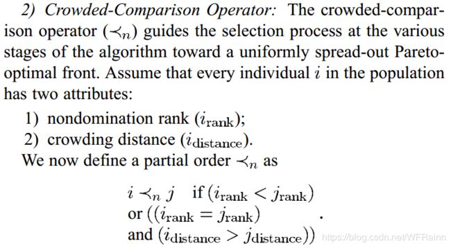
有了拥挤距离，便可以定义拥挤比较算子。简单来说，此算子的计算流程如下。对于越优的非支配曲面中的个体，其适应度函数值越大。而对于同一非支配曲面中的个体，根据拥挤距离确定适应度函数，拥挤距离越大，密度越小，适应度函数值越高。论文中描述如下：

NSGA-Ⅱ算法流程

在解释完快速非支配排序算法和拥挤比较算子后，我们便可以设计整个算法流程了。首先定义参数：定义$P_i$为第$i$代种群，而$P_0$为初始种群。种群中个体数为$N$。而$Q_i$为通过遗传算法产生的第$i$子代，数目也为$N$。算法描述如下：

1.随机产生初始代种群$P_0$，个体数为$N$
2.通过交叉算子与遗传算子得到子代$Q_0$
3.合并种群$P_0$与$Q_0$，得到个数为$2N$的种群。
4.通过快速非支配排序算法求得种群中每个个体的适应度函数。
5.通过拥挤比较算子执行自然选择过程。同时，在选择过程中引入精英机制（elitism），保留排在前面的非支配曲面。具体来说，首先保留最优非支配曲面的所有解，如果个数小于N，则继续保留第二非支配曲面的解，以此类推，直至无法保留此非支配曲面的所有解，即保留总数大于N，则运用拥挤比较算子选取适应度函数值更优的解，直至总数达到N，完成选择过程。
6.得到个体数为N的下一代种群$P_1$
7.按照模型的规定进化次数重复执行2-6步，直至完成算法。

到此为止，NSGA-Ⅱ算法就阐述完了，如果想要更深入的了解此算法，可以自行搜索论文$阅{读}^{[1]}$。接下来，我们尝试用python实现算法并运用到实际中解决特定的多目标优化问题。

Python实现NSGA-Ⅱ算法并解决多目标投资组合优化问题

模型描述

均值-方差理论自从马科维茨在1959年提出后，逐渐成为了现代投资理论的基石。在均值-方差理论中，马科维茨将资产的收益率定义为其收益率分布的均值，而将其收益率分布的方差定义为资产的风险，而资产组合的优化问题被定义为寻找收益率均值高同时方差小的投资组合。近几十年，均值-方差理论得到了多方面的发展，越来越多的目标被考虑进来，比如收益率分布的偏度与峰度，资产的流动性，熵，VaR，换手率等；另一方面，基于可信度与可能性理论的投资组合优化理论也得到充分的研究与发展。
本篇文章中， 我们具体考虑均值-方差-换手率（expectation-variance-turnover rate）投资组合模型。定义投资组合中资产$i$的比例为$x_i$，投资组合中总资产数为$n$。同时，为了模拟更为真实的投资环境，我们禁止买空操作，同时，加入Yager熵用于分散投资，并且设置投资组合中每个资产的投资上限与下限为$u$和$l$。关于这部分内容，由于不是本文重点，就不做具体阐述，有兴趣的读者可以自行查阅相关资料。这样，我们的投资组合优化模型可以表示为：

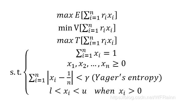
很明显，这是一个三目标的优化问题，一般需要运用启发式算法求解，这里我们采用上文阐述的NSGA-Ⅱ进行求解。

数据选取

这里我们选用深交所与上交所上市的12只股票在2014年至2016年的日交易数据，数据来源为同花顺。股票选取如下：

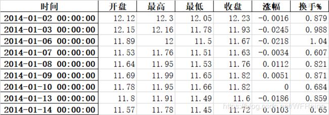
原始数据格式如下：

数据处理

接下来通过dataProcessing.py对数据进行处理：

"""
data process
"""
import pandas as pd

#define function to output processed file
def outputFile(data,source):
    data.to_excel(source+'.xlsx',encoding='utf-8')

name=['000002','600690','002001','600009','000001','002008','002236','002384','002304','600885','000046','000858']
suffix='_price'

returnData=pd.DataFrame()
turnoverData=pd.DataFrame()
for i in range(len(name)):
    data=pd.read_excel('../rowData/'+name[i]+suffix+'.xlsx')
    data.index=pd.to_datetime(data['时间'])
    returnData[name[i]]=data['涨幅']
    turnoverData[name[i]]=data['换手%']

returnData=returnData.fillna(0)
turnoverData=turnoverData.fillna(0)
outputFile(returnData,'../processedData/returns')
outputFile(turnoverData,'../processedData/turnovers')

整合所选股票日收益率与换手率数据，对于数据缺失的部分，一般为股票停牌，我们用0代替。

NSGA-Ⅱ

在NSGA2Selection.py文件中，我们首先定义3个目标的计算函数：

"""
NSGA2 selection
"""
import pandas as pd
import numpy as np

#compute the expectation of the returns of the portfolio
def expectation(returns,weights):
    eArray=np.array(returns.mean())
    return np.dot(eArray,weights.T)

#compute the variance of the returns of the portfolio
def variance(returns,weights):    
    return np.dot(weights.T, np.dot(returns.cov()*len(returns.index),weights))
    
#compute the skewness of the returns of the portfolio
def turnover(turnovers,weights):
    tArray=np.array(turnovers.mean())
    return np.dot(tArray,weights.T)

接着，定义函数用于将计算结果保存：

#generate value set for every objective
def objectiveValueSet(population,populationSize,fun,data):
    valueList=[0 for i in range(populationSize)]
    for i in range(populationSize):
        valueList[i]=fun(data,np.array(population[i][0]))
    return valueList

做完准备工作后，便可以编写快速非支配排序算法了：

#Fast Nondominated Sorting Approach
def NSGA(population,populationSize,returns,turnovers):
    #build list and compute return,variance,turnover rate for every entity in the population
    returnList=objectiveValueSet(population,populationSize,expectation,returns)
    varianceList=objectiveValueSet(population,populationSize,variance,returns)
    turnoverList=objectiveValueSet(population,populationSize,turnover,turnovers)
    
    #define the dominate set Sp
    dominateList=[set() for i in range(populationSize)]
    #define the dominated set
    dominatedList=[set() for i in range(populationSize)]
    #compute the dominate and dominated entity for every entity in the population
    for i in range(populationSize):
        for j in range(populationSize):
            if returnList[i]> returnList[j] and varianceList[i]<varianceList[j] and turnoverList[i]>turnoverList[j]:
                dominateList[i].add(j)
                
            elif returnList[i]< returnList[j] and varianceList[i]>varianceList[j] and turnoverList[i]<turnoverList[j]:
                dominatedList[i].add(j)
    #compute dominated degree Np
    for i in range(len(dominatedList)):
        dominatedList[i]=len(dominatedList[i])
    #create list to save the non-dominated front information
    NDFSet=[]
    #compute non-dominated front
    while max(dominatedList)>=0:
        front=[]
        for i in range(len(dominatedList)):
            if dominatedList[i]==0:
                front.append(i)
        NDFSet.append(front)
        for i in range(len(dominatedList)):
            dominatedList[i]=dominatedList[i]-1                                
    return NDFSet

其中，population是种群保存当前种群信息的list，大小为populationSize×2×12，其中二阶的两个长度为12的list分别用于存储12只股票的投资比例和是否投资的信息，具体定义方法将在后面提到。
dominatedList与dominateList分别用于储存种群中每个个体的支配集合与被支配度。使用set()的原因是为了避免重复添加。
最后得到的NDFSet储存着非支配曲面的信息。注意到其中会存在部分空list，这是由于支配度相差大于1所导致的，但是不影响后续建模。


接着编写拥挤距离函数：

#crowded distance
def crowdedDistance(population,Front,minmax,returns,turnovers):
    #create distance list to save the information of crowded for every entity in front
    distance=pd.Series([float(0) for i in range(len(Front))], index=Front)
    #save information of weight for every entity in front
    FrontSet=[]
    for i in Front:
        FrontSet.append(population[i])

    #compute and save objective value for every entity in front
    returnsList=objectiveValueSet(FrontSet,len(FrontSet),expectation,returns)
    varianceList=objectiveValueSet(FrontSet,len(FrontSet),variance,returns)
    turnoverList=objectiveValueSet(FrontSet,len(FrontSet),turnover,turnovers)   
    returnsSer=pd.Series(returnsList,index=Front)
    varianceSer=pd.Series(varianceList,index=Front)
    turnoverSer=pd.Series(turnoverList,index=Front)
    #sort value
    returnsSer.sort_values(ascending=False,inplace=True)
    varianceSer.sort_values(ascending=False,inplace=True)
    turnoverSer.sort_values(ascending=False,inplace=True)
    #set the distance for the entities which have the min and max value in every objective 
    distance[returnsSer.index[0]]=1000
    distance[returnsSer.index[-1]]=1000
    distance[varianceSer.index[0]]=1000
    distance[varianceSer.index[-1]]=1000
    distance[turnoverSer.index[0]]=1000
    distance[turnoverSer.index[-1]]=1000
    for i in range(1,len(Front)-1):
        distance[returnsSer.index[i]]=distance[returnsSer.index[i]]+(returnsSer[returnsSer.index[i-1]]-returnsSer[returnsSer.index[i+1]])/(minmax.iloc[0,1]-minmax.iloc[0,0])
        distance[varianceSer.index[i]]+=(varianceSer[varianceSer.index[i-1]]-varianceSer[varianceSer.index[i+1]])/(minmax.iloc[1,1]-minmax.iloc[1,0])
        distance[turnoverSer.index[i]]+=(turnoverSer[turnoverSer.index[i-1]]-turnoverSer[turnoverSer.index[i+1]])/(minmax.iloc[2,1]-minmax.iloc[2,0])
    distance.sort_values(ascending=False,inplace=True)
    return distance

这里由于使用无穷大不方便计算，使用1000作为无穷大的代替。minmax里储存着每个目标的最大值与最小值，用于标准化每个目标值，对于一阶矩，可直接进行计算，对于二阶矩方差使用单目标遗传算法得到近似结果，具体代码便不赘述了，具体可仿照本人之前的文章编写。


有了计算拥挤距离的函数，接下来编写拥挤比较算子：

def crowdedCompareOperator(population,populationSize,NDFSet,minmax,returns,turnovers):
    newPopulation=[]
    #save the information of the entity the new population have
    count=0
    #save the information of the succession of the front 
    number=0
    while count<populationSize:            
        if count + len(NDFSet[number])<=populationSize:
            if number==0:
                #save the information of the first non-dominated front
                firstFront=[i for i in range(len(NDFSet[number]))]
            for i in NDFSet[number]:
                newPopulation.append(population[i])
            count+=len(NDFSet[number])
            number+=1
        else:
            if number==0:
                firstFront=[i for i in range(populationSize)]
            n=populationSize-count
            distance=crowdedDistance(population,NDFSet[number],minmax,returns,turnovers)
            for i in range(n):
                newPopulation.append(population[distance.index[i]])
            number+=1
            count+=n

    return newPopulation,firstFront

这里firstFront用于储存自然选择后种群中处于最优非支配曲面上的个体，因为最后进行分析时一般只需要用到最优分支配曲面。


接下来编写选择主函数：

def NSGA2Selection(population,populationSize,minmax,returns,turnovers):
    NDFSet=NSGA(population,populationSize*2,returns,turnovers)
    newPopulation,firstFront=crowdedCompareOperator(population,populationSize,NDFSet,minmax,returns,turnovers)
    return newPopulation,firstFront,NDFSet

有了NSGA2选择算子，我们接着编写遗传算法主函数文件。不过首先我们在tools.py定义工具函数

"""
function tools
"""


#initiate stock list signal
def stocksignal(population,populationSize):
    for i in range(populationSize):
        stocklist=[]
        for j in range(12):
            if population[i][0][j]>0:
                stocklist.append(1)
            else:
                stocklist.append(0)
        if len(population[i])==1:
            population[i].append(stocklist)
        else:
            population[i][1]=stocklist
    return population

def yagersEntropy(porprotion,n):
    H=0
    for i in range(n):
        H+=abs(porprotion[i]-1/n)
        
    return H

其中stocksignal函数用于计算是否投资某个具体股票，投资则为1，为投资则为0，此信息在交叉与遗传算子中将会用到。yagersEntropy函数用于计算投资组合的雅各熵。


编写主函数文件multiObjective.py,首先导入各算子模块并定义参数：

import pandas as pd
import tools
import random
from crossover import crossover
from mutation import mutation
from repair import repair
from NSGA2Selection import NSGA2Selection

returns=pd.read_excel('../processedData/returns.xlsx')
turnovers=pd.read_excel('../processedData/turnovers.xlsx')
minmax=pd.read_excel('../processedData/minmaxValue.xlsx')

populationSize=50
generation=50
Pm=0.5
Pc=0.9
l=0.05
u=0.3

crossover与mutation模块为交叉与变异算子，但由于研究问题不公布在上面，有兴趣的读者可以自行查阅文献按照相关规则设计。repair模块为修复算子，用于在交叉与变异后调整比例使得投资组合重新满足各项限制（如最大最小值，雅阁熵），由于研究问题同样就不公布了，设计起来其实也不是很难，相关文献也有很多。
Pm为变异概率，为了提高种群多样性与避免局部最小值，将变异概率调高至0.5；Pc为交叉概率，l与u分别为每只股票所能投资的下限与上限。


接着初始化种群：

#initiate population    
population=[[] for i in range(populationSize)]
selectedPopulation=[[] for i in range(populationSize)]
for i in range(populationSize):
    entity=[0 for i in range(12)]
    n=1
    label=[i for i in range(12)]
    for j in range(12):
        if n>u:
            t=random.choice(label)
            entity[t]=random.uniform(l,u)
            n-=entity[t]
            label.remove(t)
        elif n<l:            
            entity[t]+=n
            n=0
        else:
            t=random.choice(label)
            entity[t]=random.uniform(l,n)
            n-=entity[t]         
            label.remove(t)              
    population[i].append(entity)
    selectedPopulation[i].append(entity)
newPopulation=tools.stocksignal(population,populationSize)

执行循环：

#GA loop
for i in range(generation):
    offspring=crossover(newPopulation,populationSize,Pc,l,u)
    offspring=mutation(offspring,populationSize,Pm)
    offspring=repair(offspring,populationSize,l,u)
    selectPopulation=selectedPopulation+offspring
    selectedPopulation,firstFront,NDFSet=NSGA2Selection(selectPopulation,populationSize,minmax,returns,turnovers)
    newPopulation=tools.stocksignal(selectedPopulation,populationSize)
    print (i)

如果执行循环可以发现，最优非支配面上的个体将逐渐增加，证明通过遗传算法种群在不断进行优化。


完成循环后，储存最优非支配面上个体的信息并保存以做后续分析：

name=['000002','600690','002001','600009','000001','002008','002236','002384','002304','600885','000046','000858']
result=pd.DataFrame([[0 for j in range(len(name))] for i in range(len(firstFront))])
for i in range(len(firstFront)):
    for j in range(len(name)):
        result.iloc[i,j]=newPopulation[firstFront[i]][0][j]

result.columns=name
result.to_excel('../resultData/result2.xlsx',encoding='utf-8')

这样，我们便使用NSGA-Ⅱ算法解决了多目标投资组合优化问题，对于得到的结果，我们可以通过运用历史数据进行回测评价效果，具体便不赘述。
相关代码与数据已经上传至Github，由于编写仓促，代码有许多不完善的地方，欢迎大家进行讨论！

[1]Deb, Kalyanmoy, Pratap, Amrit, Agarwal, Sameer, et al. A fast and elitist multiobjective genetic algorithm: NSGA-II[J]. IEEE Transactions on Evolutionary Computation, 2002, 6(2):182-197.