实战 | Kaggle竞赛:预测二手车每年平均价值损失
点击标题下「蓝色微信名」可快速关注
本文所有代码都通过运行!
目录:
1、准备数据
2、清洗数据
3、可视化
4、特征工程
5、关联性分析
6、准备模型
7、随机森林
本项目带你根据以上过程带你完成Kaggle挑战之旅!
01
准备数据
数据集:
Ebay-Kleinanzeigen二手车数据集
[有超过370000辆二手车的相关数据]
数据字段说明:
dateCrawled :当这个广告第一次被抓取日期
name :车的名字
seller : 私人或经销商
offerType
price : 价格
abtest:测试
vehicleType:车辆类型
yearOfRegistration :车辆首次注册年份
gearbox:变速箱
powerPS : 汽车在PS中的功率
model:型号
kilometer : 已经行驶的里程数
monthOfRegistration : 车辆首次注册的月份
fuelType:燃料类型
brand:品牌
notRepairedDamage :车辆有损坏还没修复
dateCreated :在ebay首次创建广告的时间
nrOfPictures :广告中的图片数量
postalCode:邮政编码
lastSeenOnline :当爬虫最后在网上看到这个广告的时候
数据来源:
https://www.kaggle.com/orgesleka/used-cars-database
代码:
1import pandas as pd
2import matplotlib.pyplot as plt
3import numpy as np
4from sklearn import datasets, linear_model, preprocessing, svm
5from sklearn.preprocessing import StandardScaler, Normalizer
6import math
7import matplotlib
8import seaborn as sns
9df = pd.read_csv('../autos.csv')
02
清洗数据
代码:
 1#让我们看看数字字段中的一些信息
 2df.describe()
 3
 4#丢弃一些无用的列
 5df.drop(['seller', 'offerType', 'abtest', 'dateCrawled', 'nrOfPictures', 'lastSeen', 'postalCode', 'dateCreated'], axis='columns', inplace=True)
 6
 7#从重复的、NAN中清除数据并为列选择合理的范围
 8print("Too new: %d" % df.loc[df.yearOfRegistration >= 2017].count()['name'])
 9print("Too old: %d" % df.loc[df.yearOfRegistration < 1950].count()['name'])
10print("Too cheap: %d" % df.loc[df.price < 100].count()['name'])
11print("Too expensive: " , df.loc[df.price > 150000].count()['name'])
12print("Too few km: " , df.loc[df.kilometer < 5000].count()['name'])
13print("Too many km: " , df.loc[df.kilometer > 200000].count()['name'])
14print("Too few PS: " , df.loc[df.powerPS < 10].count()['name'])
15print("Too many PS: " , df.loc[df.powerPS > 500].count()['name'])
16print("Fuel types: " , df['fuelType'].unique())
17#print("Offer types: " , df['offerType'].unique())
18#print("Sellers: " , df['seller'].unique())
19print("Damages: " , df['notRepairedDamage'].unique())
20#print("Pics: " , df['nrOfPictures'].unique()) # nrOfPictures : number of pictures in the ad (unfortunately this field contains everywhere a 0 and is thus useless (bug in crawler!) )
21#print("Postale codes: " , df['postalCode'].unique())
22print("Vehicle types: " , df['vehicleType'].unique())
23print("Brands: " , df['brand'].unique())
24
25# Cleaning data
26#valid_models = df.dropna()
27
28#### Removing the duplicates
29dedups = df.drop_duplicates(['name','price','vehicleType','yearOfRegistration'
30                         ,'gearbox','powerPS','model','kilometer','monthOfRegistration','fuelType'
31                         ,'notRepairedDamage'])
32
33#### Removing the outliers
34dedups = dedups[
35        (dedups.yearOfRegistration <= 2016)
36      & (dedups.yearOfRegistration >= 1950)
37      & (dedups.price >= 100)
38      & (dedups.price <= 150000)
39      & (dedups.powerPS >= 10)
40      & (dedups.powerPS <= 500)]
41
42print("-----------------\nData kept for analisys: %d percent of the entire set\n-----------------" % (100 * dedups['name'].count() / df['name'].count()))
输出:

处理空值:
1dedups.isnull().sum()
2dedups['notRepairedDamage'].fillna(value='not-declared', inplace=True)
3dedups['fuelType'].fillna(value='not-declared', inplace=True)
4dedups['gearbox'].fillna(value='not-declared', inplace=True)
5dedups['vehicleType'].fillna(value='not-declared', inplace=True)
6dedups['model'].fillna(value='not-declared', inplace=True)
03
可视化
让我们看看一些图表,以了解数据是如何跨类别分布的。
代码:
 1categories = ['gearbox', 'model', 'brand', 'vehicleType', 'fuelType', 'notRepairedDamage']
 2
 3for i, c in enumerate(categories):
 4    v = dedups[c].unique()
 5
 6    g = dedups.groupby(by=c)[c].count().sort_values(ascending=False)
 7    r = range(min(len(v), 5))
 8
 9    print( g.head())
10    plt.figure(figsize=(5,3))
11    plt.bar(r, g.head())
12    #plt.xticks(r, v)
13    plt.xticks(r, g.index)
14    plt.show()
输出(拿其中一个输出为例):

04
特征工程
添加名称长度以查看长描述对价格的影响有多大
代码:
1dedups['namelen'] = [min(70, len(n)) for n in dedups['name']]
2
3ax = sns.jointplot(x='namelen',
4                   y='price',
5                   data=dedups[['namelen','price']],
6#                   data=dedups[['namelen','price']][dedups['model']=='golf'],
7                    alpha=0.1,
8                    size=8)
输出:

似乎在15到30个字符之间的名字长度是更好的销售价格。一个解释可能是一个较长的名称包括更多的选择和配件,因此价格显然更高。很短的名字和很长的名字不能很好的工作。
代码:
 1labels = ['name', 'gearbox', 'notRepairedDamage', 'model', 'brand', 'fuelType', 'vehicleType']
 2les = {}
 3
 4for l in labels:
 5    les[l] = preprocessing.LabelEncoder()
 6    les[l].fit(dedups[l])
 7    tr = les[l].transform(dedups[l])
 8    dedups.loc[:, l + '_feat'] = pd.Series(tr, index=dedups.index)
 9
10labeled = dedups[ ['price'
11                        ,'yearOfRegistration'
12                        ,'powerPS'
13                        ,'kilometer'
14                        ,'monthOfRegistration'
15                        , 'namelen']
16                    + [x+"_feat" for x in labels]]
17len(labeled['name_feat'].unique()) / len(labeled['name_feat'])
18#输出:0.6224184813880769
19#name列的标签占总数的62%。我觉得太多了,所以我删除了这个特征。
20labeled.drop(['name_feat'], axis='columns', inplace=True)
05
关联性分析
让我们看看功能如何相互关联,更重要的是,与价格。
代码:
1#所有属性间的关联
2plot_correlation_map(labeled)
3labeled.corr()
4labeled.corr().loc[:,'price'].abs().sort_values(ascending=False)[1:]
输出:
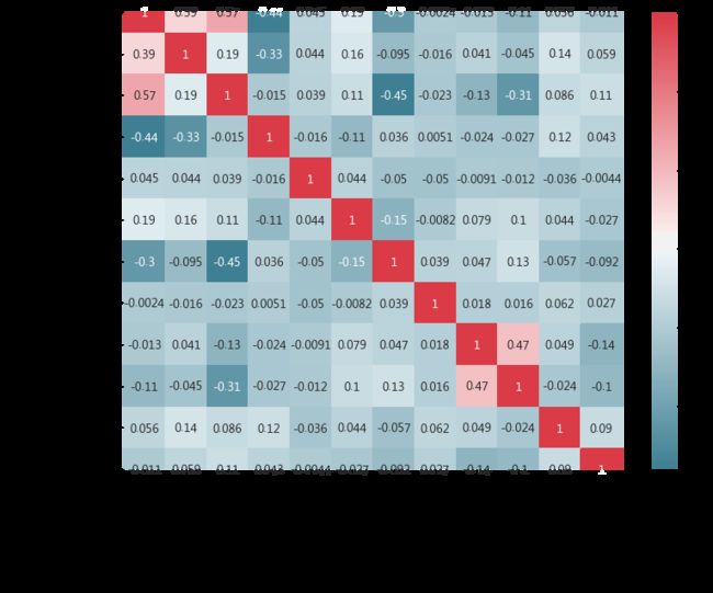

相关性是指两个变量的观测值之间的关联。变量可能有正相关,即当一个变量的值增加时,另一个变量的值也会增加。也可能有负相关,意味着随着一个变量的值增加,其他变量的值减小。变量也可能是中立的,也就是说变量不相关。相关性的量化通常为值-1到1之间的度量,即完全负相关和完全正相关。计算出的相关结果被称为“ 相关系数”。然后可以解释该相关系数以描述度量。
06
准备模型
代码:
1Y = labeled['price']
2X = labeled.drop(['price'], axis='columns', inplace=False)
3matplotlib.rcParams['figure.figsize'] = (12.0, 6.0)
4prices = pd.DataFrame({"1. Before":Y, "2. After":np.log1p(Y)})
5prices.hist()
7Y = np.log1p(Y)
输出:

代码:
 1from sklearn.linear_model import Ridge, RidgeCV, ElasticNet, Lasso, LassoCV, LassoLarsCV
 2from sklearn.model_selection import cross_val_score, train_test_split
 3
 4def cv_rmse(model, x, y):
 5    r = np.sqrt(-cross_val_score(model, x, y, scoring="neg_mean_squared_error", cv = 5))
 6    return r
 7
 8# Percent of the X array to use as training set. This implies that the rest will be test set
 9test_size = .33
10
11#Split into train and validation
12X_train, X_val, y_train, y_val = train_test_split(X, Y, test_size=test_size, random_state = 3)
13print(X_train.shape, X_val.shape, y_train.shape, y_val.shape)
14
15r = range(2003, 2017)
16km_year = 10000
07
随机森林
我使用GridSearch为回归器设置最优参数,然后训练最终的模型。我已经删除了其他参数,以便在脱机处理许多参数时快速地将这一点传递到网上。
代码:
 1from sklearn.ensemble import RandomForestRegressor
 2from sklearn.model_selection import GridSearchCV
 3
 4rf = RandomForestRegressor()
 5
 6param_grid = { "criterion" : ["mse"]
 7              , "min_samples_leaf" : [3]
 8              , "min_samples_split" : [3]
 9              , "max_depth": [10]
10              , "n_estimators": [500]}
11
12gs = GridSearchCV(estimator=rf, param_grid=param_grid, cv=2, n_jobs=-1, verbose=1)
13gs = gs.fit(X_train, y_train)
14print(gs.best_score_)
15print(gs.best_params_)
16bp = gs.best_params_
17forest = RandomForestRegressor(criterion=bp['criterion'],
18                              min_samples_leaf=bp['min_samples_leaf'],
19                              min_samples_split=bp['min_samples_split'],
20                              max_depth=bp['max_depth'],
21                              n_estimators=bp['n_estimators'])
22forest.fit(X_train, y_train)
运行最后得分为0.83!试试看?


135编辑器
客官!在看一下呗~