可解释机器学习-shap value的使用

1 数据预处理和建模

1.1 加载库和数据预处理

import pandas as pd
import numpy as np
from sklearn.metrics import roc_auc_score, precision_recall_curve, roc_curve, average_precision_score
from sklearn.model_selection import KFold, train_test_split
from lightgbm import LGBMClassifier
import matplotlib.pyplot as pl
import gc # 对已经销毁的对象,Python不会自动释放其占据的内存空间。为了能够充分地利用分配的内存,避免程序跑到一半停止,要时不时地进行内存回收
import shap

file_path = 'D:\\jupyter files\\shap_value_practice_data\\home-credit-default-risk\\'

def build_model_input():
    buro_bal = pd.read_csv(file_path + 'bureau_balance.csv')
    print('Buro bal shape : ', buro_bal.shape)
    
    print('transform to dummies')
    buro_bal = pd.concat([buro_bal, pd.get_dummies(buro_bal.STATUS, prefix='buro_bal_status')], axis=1).drop('STATUS', axis=1)
    
    print('Counting buros')
    buro_counts = buro_bal[['SK_ID_BUREAU', 'MONTHS_BALANCE']].groupby('SK_ID_BUREAU').count()
    buro_bal['buro_count'] = buro_bal['SK_ID_BUREAU'].map(buro_counts['MONTHS_BALANCE'])
    
    print('averaging buro bal')
    avg_buro_bal = buro_bal.groupby('SK_ID_BUREAU').mean()
    
    avg_buro_bal.columns = ['avg_buro_' + f_ for f_ in avg_buro_bal.columns]
    del buro_bal
    gc.collect()
    
    print('Read Bureau')
    buro = pd.read_csv(file_path + 'bureau.csv')
    
    print('Go to dummies')
    buro_credit_active_dum = pd.get_dummies(buro.CREDIT_ACTIVE, prefix='ca_')
    buro_credit_currency_dum = pd.get_dummies(buro.CREDIT_CURRENCY, prefix='cu_')
    buro_credit_type_dum = pd.get_dummies(buro.CREDIT_TYPE, prefix='ty_')
    
    buro_full = pd.concat([buro, buro_credit_active_dum, buro_credit_currency_dum, buro_credit_type_dum], axis=1)
    # buro_full.columns = ['buro_' + f_ for f_ in buro_full.columns]
    
    del buro_credit_active_dum, buro_credit_currency_dum, buro_credit_type_dum
    gc.collect()
    
    print('Merge with buro avg')
    buro_full = buro_full.merge(right=avg_buro_bal.reset_index(), how='left', on='SK_ID_BUREAU', suffixes=('', '_bur_bal'))
    
    print('Counting buro per SK_ID_CURR')
    nb_bureau_per_curr = buro_full[['SK_ID_CURR', 'SK_ID_BUREAU']].groupby('SK_ID_CURR').count()
    buro_full['SK_ID_BUREAU'] = buro_full['SK_ID_CURR'].map(nb_bureau_per_curr['SK_ID_BUREAU'])
    
    print('Averaging bureau')
    avg_buro = buro_full.groupby('SK_ID_CURR').mean()
    print(avg_buro.head())
    
    del buro, buro_full
    gc.collect()
    
    print('Read prev')
    prev = pd.read_csv(file_path + 'previous_application.csv')
    
    prev_cat_features = [
        f_ for f_ in prev.columns if prev[f_].dtype == 'object'
    ]
    
    print('Go to dummies')
    prev_dum = pd.DataFrame()
    for f_ in prev_cat_features:
        prev_dum = pd.concat([prev_dum, pd.get_dummies(prev[f_], prefix=f_).astype(np.uint8)], axis=1)
    
    prev = pd.concat([prev, prev_dum], axis=1)
    
    del prev_dum
    gc.collect()
    
    print('Counting number of Prevs')
    nb_prev_per_curr = prev[['SK_ID_CURR', 'SK_ID_PREV']].groupby('SK_ID_CURR').count()
    prev['SK_ID_PREV'] = prev['SK_ID_CURR'].map(nb_prev_per_curr['SK_ID_PREV'])
    
    print('Averaging prev')
    avg_prev = prev.groupby('SK_ID_CURR').mean()
    #print(avg_prev.head())
    del prev
    gc.collect()
    
    print('Reading POS_CASH')
    pos = pd.read_csv(file_path + 'POS_CASH_balance.csv')
    
    print('Go to dummies')
    pos = pd.concat([pos, pd.get_dummies(pos['NAME_CONTRACT_STATUS'])], axis=1)
    
    print('Compute nb of prevs per curr')
    nb_prevs = pos[['SK_ID_CURR', 'SK_ID_PREV']].groupby('SK_ID_CURR').count()
    pos['SK_ID_PREV'] = pos['SK_ID_CURR'].map(nb_prevs['SK_ID_PREV'])
    
    print('Go to averages')
    avg_pos = pos.groupby('SK_ID_CURR').mean()
    
    del pos, nb_prevs
    gc.collect()
    
    print('Reading CC balance')
    cc_bal = pd.read_csv(file_path + 'credit_card_balance.csv')
    
    print('Go to dummies')
    cc_bal = pd.concat([cc_bal, pd.get_dummies(cc_bal['NAME_CONTRACT_STATUS'], prefix='cc_bal_status_')], axis=1)
    
    nb_prevs = cc_bal[['SK_ID_CURR', 'SK_ID_PREV']].groupby('SK_ID_CURR').count()
    cc_bal['SK_ID_PREV'] = cc_bal['SK_ID_CURR'].map(nb_prevs['SK_ID_PREV'])
    
    print('Compute average')
    avg_cc_bal = cc_bal.groupby('SK_ID_CURR').mean()
    avg_cc_bal.columns = ['cc_bal_' + f_ for f_ in avg_cc_bal.columns]
    
    del cc_bal, nb_prevs
    gc.collect()
    
    print('Reading Installments')
    inst = pd.read_csv(file_path + 'installments_payments.csv')
    nb_prevs = inst[['SK_ID_CURR', 'SK_ID_PREV']].groupby('SK_ID_CURR').count()
    inst['SK_ID_PREV'] = inst['SK_ID_CURR'].map(nb_prevs['SK_ID_PREV'])
    
    avg_inst = inst.groupby('SK_ID_CURR').mean()
    avg_inst.columns = ['inst_' + f_ for f_ in avg_inst.columns]
    
    print('Read data and test')
    data = pd.read_csv(file_path + 'application_train.csv')
    test = pd.read_csv(file_path + 'application_test.csv')
    print('Shapes : ', data.shape, test.shape)
    
    y = data['TARGET']
    del data['TARGET']
    
    categorical_feats = [
        f for f in data.columns if data[f].dtype == 'object'
    ]
    categorical_feats
    for f_ in categorical_feats:
        data[f_], indexer = pd.factorize(data[f_])
        test[f_] = indexer.get_indexer(test[f_])
        
    data = data.merge(right=avg_buro.reset_index(), how='left', on='SK_ID_CURR')
    test = test.merge(right=avg_buro.reset_index(), how='left', on='SK_ID_CURR')
    
    data = data.merge(right=avg_prev.reset_index(), how='left', on='SK_ID_CURR')
    test = test.merge(right=avg_prev.reset_index(), how='left', on='SK_ID_CURR')
    
    data = data.merge(right=avg_pos.reset_index(), how='left', on='SK_ID_CURR')
    test = test.merge(right=avg_pos.reset_index(), how='left', on='SK_ID_CURR')
    
    data = data.merge(right=avg_cc_bal.reset_index(), how='left', on='SK_ID_CURR')
    test = test.merge(right=avg_cc_bal.reset_index(), how='left', on='SK_ID_CURR')
    
    data = data.merge(right=avg_inst.reset_index(), how='left', on='SK_ID_CURR')
    test = test.merge(right=avg_inst.reset_index(), how='left', on='SK_ID_CURR')
    
    del avg_buro, avg_prev
    gc.collect()

    return data, test, y

训练的时候，出现了因为json 字符无法加载的相关报错。原因是特征名称里，包含着比如（ +这一类的特殊符号。

因此，我把特征名称只保留了中英文和数字。

import re
def get_name(name):
    cop = re.compile("[^\u4e00-\u9fa5^a-z^A-Z^0-9]") # 匹配不是中文、大小写、数字的其他字符
    new_name = cop.sub('', name) #将name 中匹配到的字符替换成空字符
    return new_name

处理数据，拆分训练集和测试集。

data, test, y = build_model_input()

new_name_list = [get_name(name) for name in list(data.columns)]
data.columns = new_name_list

data_train, data_valid, y_train, y_valid = train_test_split(data, y, test_size=0.2, random_state=0)

1.2 训练

使用lightgbm 模型进行训练。

clf = LGBMClassifier(
    n_estimators=400,
    learning_rate=0.03,
    num_leaves=30,
    colsample_bytree=.8,
    subsample=.9,
    max_depth=7,
    reg_alpha=.1,
    reg_lambda=.1,
    min_split_gain=.01,
    min_child_weight=2,
    silent=-1,
    verbose=-1,
)

clf.fit(
    data_train, y_train, 
    eval_set= [(data_train, y_train), (data_valid, y_valid)], 
    eval_metric='auc', verbose=100, early_stopping_rounds=30
)
# verbose 这个参数是控制多少轮打印一次结果。

[output]:
Training until validation scores don't improve for 30 rounds
[100]	training's auc: 0.779201	training's binary_logloss: 0.242767	valid_1's auc: 0.763555	valid_1's binary_logloss: 0.242803
[200]	training's auc: 0.800839	training's binary_logloss: 0.233891	valid_1's auc: 0.775869	valid_1's binary_logloss: 0.238003
[300]	training's auc: 0.814925	training's binary_logloss: 0.228279	valid_1's auc: 0.78042	valid_1's binary_logloss: 0.236285
[400]	training's auc: 0.826468	training's binary_logloss: 0.223792	valid_1's auc: 0.782228	valid_1's binary_logloss: 0.235568
Did not meet early stopping. Best iteration is:
[400]	training's auc: 0.826468	training's binary_logloss: 0.223792	valid_1's auc: 0.782228	valid_1's binary_logloss: 0.235568

2 解释模型

首先，把需要解释的这部分数据，输入到shap 中。

# explain 10000 examples from the validation set
# each row is an explanation for a sample, and the last column in the base rate of the model
# the sum of each row is the margin (log odds) output of the model for that sample

shap_values = shap.TreeExplainer(clf.booster_).shap_values(data_valid.iloc[:10000,:])
print('length of shape: ', len(shap_values))
print('y: ', set(y))

[output]:
length of shape:  2
y:  {0, 1}

需要注意的是，shap输出的是每一个样本中，每一个特征对于模型输出的影响，输出为矩阵形式。

对于分类问题，如二分类，shap 会输出两个矩阵，分别对应着两个标签。两个矩阵内的值为相反数。多分类的话，也会有多个矩阵，不过里面的值没有这种相反数的关系，多分类的情况见下文。

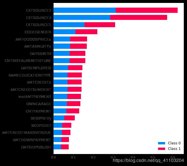
2.1 Summarize the feature imporances with a bar chart

特征的整体影响。对于每一个样本，不同特征对于模型影响的绝对平均值。

# compute the global importance of each feature as the mean absolute value
# of the feature's importance over all the samples
global_importances = np.abs(shap_values).mean(0)[:-1]

[output]:
global_importances

array([[3.70270513e-04, 1.11664905e-02, 8.02847521e-02, ...,
        3.11673525e-03, 1.92387261e-03, 3.95504321e-02],
       [3.38818783e-04, 1.73549029e-02, 1.70608421e-01, ...,
        9.61602884e-04, 3.20387773e-03, 7.76451402e-02],
       [6.00685043e-04, 2.13988061e-01, 1.11142791e-01, ...,
        1.43808390e-02, 2.82810665e-03, 6.64158636e-03],
       ...,
       [2.34631684e-04, 1.06669623e-02, 2.42689718e-01, ...,
        3.34426851e-03, 6.75652200e-04, 4.48376155e-02],
       [7.58788691e-04, 9.22195270e-02, 5.70158483e-02, ...,
        1.05911300e-02, 1.09188272e-02, 5.77955976e-03],
       [6.54479612e-04, 9.04468726e-02, 7.60136842e-02, ...,
        4.86721485e-03, 8.20539474e-04, 9.53252329e-02]])

对于分类问题，如果我们将几个标签对应的矩阵都画出来，就会出现下面这个图的样子，每种颜色对应一类标签。

shap.summary_plot(shap_values, data_valid.iloc[:10000,:])

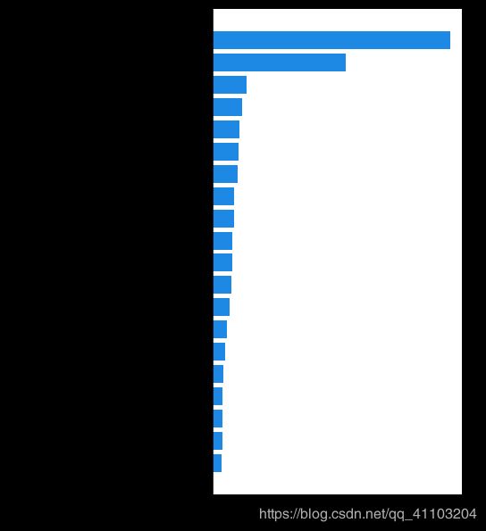
选择具体的标签所对应的矩阵，就是下面这个图的样子。

# make a bar chart that shows the global importance of the top 20 features
inds = np.argsort(-global_importances[0])
f = pl.figure(figsize=(5,10))
y_pos = np.arange(20)
inds2 = np.flip(inds[:20], 0)
pl.barh(y_pos, global_importances[0][inds2], align='center', color="#1E88E5")
pl.yticks(y_pos, fontsize=13)
pl.gca().set_yticklabels(data.columns[inds2])
pl.xlabel('mean abs. SHAP value (impact on model output)', fontsize=13)
pl.gca().xaxis.set_ticks_position('bottom')
pl.gca().yaxis.set_ticks_position('none')
pl.gca().spines['right'].set_visible(False)
pl.gca().spines['top'].set_visible(False)

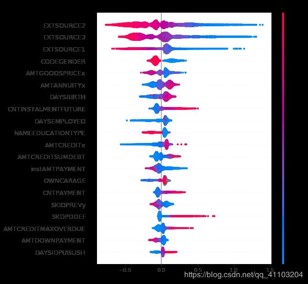
2.2 Summarize the feature importances with a density scatter plot

密度散点图画出了所有样本的情况。特征的排序是按照shap 的平均绝对值，对模型来说的最重要特征。宽的地方表示有大量的样本聚集。右边的颜色表示特征的值的大小，红色表示特征值高，蓝色表示特征值低。

比如，对于EXTSOURCE2 来说，EXTSOURCE2 的值越高，那么就会更可能令模型输出值越小（shap value 为负）。同理，如果EXTSOURCE2 的值越低，那么就会更可能令模型输出值越大（shap value 为正）。图中EXTSOURCE2 的样本大量在shap value 为负的区域聚集。

需要注意的是，一些特征，比如SKDPDDEF 对于大多数人并不是重要特征。但是可能对于某一小部分人群非常重要。我们的图只是代表全局的情况，并能不是每个人的情况

shap.summary_plot(shap_values[1], data_valid.iloc[:10000,:])

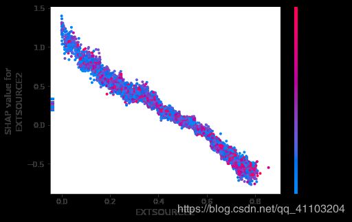
2.3 Investigate the dependence of the model on each feature

这个图显示了更加清楚的特征对于模型输出的影响。

x 轴表示特征的取值，y 值表示特征的shap value 值，也就是特征的取值，对于模型的输出会带来的变化量。其中我们可以发现对于同一个x 值，也就是特征取值相同的样本，它们的shap value不同。其原因是，该特征和其他特征有着交互相应

dependence_plot 可以自动选择另外一种特征，来表现这种交互效应。

使用interaction_index = “auto”, None, or int，可以选择某一个具体特征来着色。比如，对于 EXTSOURCE2 相同的样本，CODEGENDER 越大（红色），比越小（蓝色）带来的对模型输出的变化更大（shap value 更大）。

shap.dependence_plot("EXTSOURCE2", shap_values[1], data_valid.iloc[:10000,:], interaction_index = 7)

默认情况下，interaction_index = ‘auto’，会选择令颜色的离散程度最大的特征来进行着色。

shap.dependence_plot("EXTSOURCE2", shap_values[1], data_valid.iloc[:10000,:])

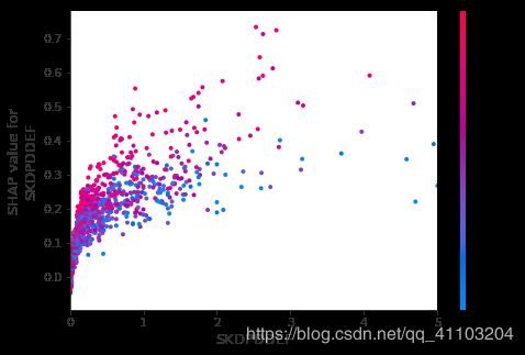
shap.dependence_plot("SKDPDDEF", shap_values[1], data_valid.iloc[:10000,:], show=False)
pl.xlim(0,5)
pl.show()

使用show=False，pl.xlim(0,5) 的原因是，由于部分样本偏离整体数据过大，全部显示很难看出数据分布情况，因此只显示0- 5 范围的数据。

2.4 Plot the SHAP dependence plots for the top 20 features

for i in reversed(inds2):
    shap.dependence_plot(i, shap_values[1], data_valid.iloc[:10000,:])

3 多变量分类

import sklearn
from sklearn.model_selection import train_test_split
import numpy as np
import shap
import time
import xgboost

X_train,X_test,Y_train,Y_test = train_test_split(*shap.datasets.iris(), test_size=0.2, random_state=0)

shap.initjs()

model = xgboost.XGBClassifier(objective="binary:logistic", max_depth=4, n_estimators=10)
model.fit(X_train, Y_train)

shap_values = shap.TreeExplainer(model).shap_values(X_test)
set(Y_train)

[output]:
{0, 1, 2}

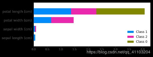
有三种标签，因此图中有三个颜色。

shap.summary_plot(shap_values, X_test)

4 lightgbm-shap 分类变量（categorical feature）的处理

在lightgbm模型里面，我们可以直接对分类变量进行处理，而不用进行编码（OneHotEncoder 或者OrdinalEncoder）。只需要我们在处理分类变量的时候，将其格式改成df[col] = df[col].astype('category')，就可以直接进行训练。

训练好后，我们也可以用shap 来对模型进行解释。

shap_values = shap.TreeExplainer(gbm.booster_).shap_values(train_x)

但是不能正常使用shap.dependence_plot()。

shap.dependence_plot("area", shap_values, train_x, display_features=train_x)

出现下面的报错。

ValueError: could not convert string to float: 'unknown'

这是因为shap 不能直接对lightgbm 里面的字符类型的分类变量进行处理。

因此，为了正常使用shap的功能，更好地办法是对分类变量采用OrdinalEncoder 编码，然后在画图的时候，加入原先变量的名称。

X,y = shap.datasets.adult()
X_display,y_display = shap.datasets.adult(display=True)

# create a train/test split
X_train, X_test, y_train, y_test = train_test_split(X, y, test_size=0.2, random_state=7)
d_train = lgb.Dataset(X_train, label=y_train)
d_test = lgb.Dataset(X_test, label=y_test)

其中，我们可以观察X_train和X_display。

X_train.head()

[output]:

Age	Workclass	Education-Num	Marital Status	Occupation	Relationship	Race	Sex	Capital Gain	Capital Loss	Hours per week	Country
12011	51.0	4	10.0	0	6	0	4	0	0.0	0.0	40.0	21
23599	51.0	1	14.0	6	12	1	4	1	0.0	0.0	50.0	8
23603	21.0	4	11.0	4	3	3	2	1	0.0	0.0	40.0	39
6163	25.0	4	10.0	4	12	3	4	1	0.0	0.0	24.0	39
14883	48.0	4	13.0	0	1	3	4	1	0.0	0.0	38.0	39

X_display.head()

[output]:
	Age	Workclass	Education-Num	Marital Status	Occupation	Relationship	Race	Sex	Capital Gain	Capital Loss	Hours per week	Country
0	39.0	State-gov	13.0	Never-married	Adm-clerical	Not-in-family	White	Male	2174.0	0.0	40.0	United-States
1	50.0	Self-emp-not-inc	13.0	Married-civ-spouse	Exec-managerial	Husband	White	Male	0.0	0.0	13.0	United-States
2	38.0	Private	9.0	Divorced	Handlers-cleaners	Not-in-family	White	Male	0.0	0.0	40.0	United-States
3	53.0	Private	7.0	Married-civ-spouse	Handlers-cleaners	Husband	Black	Male	0.0	0.0	40.0	United-States
4	28.0	Private	13.0	Married-civ-spouse	Prof-specialty	Wife	Black	Female	0.0	0.0	40.0	Cuba

4.1 Visualize a single prediction

shap.force_plot(explainer.expected_value[1], shap_values[1][0,:], X_display.iloc[0,:])

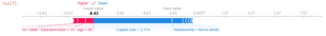
shap.force_plot(explainer.expected_value[1], shap_values[1][3,:], X_display.iloc[3,:])

这个图表示一个样本的解释图。显示不同特征对于模型输出的贡献，也就是偏离base value 的贡献。base value 是模型在整个训练样本的平均输出。红色的特征让输出结果增加，蓝色的特征让输出结果减小。

需要注意的是，我们为了能够表示分类变量的值，而不是编码后的结果，需要添加这一句X_display.iloc[3,:]。

4.2 Visualize whole dataset prediction

shap.force_plot(explainer.expected_value[1], shap_values[1][:1000,:], X_display.iloc[:1000,:])

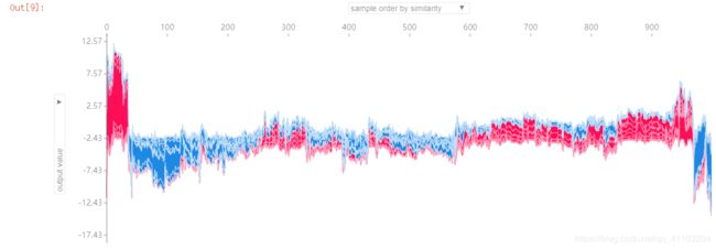
如果我们把上面的一个样本的解释图旋转90°，然后水平的堆积起所有的样本，就会出现上面的图片。这是全样本的解释图，我们可以选择不同的横纵坐标。

4.3 SHAP Summary Plot

shap.summary_plot(shap_values[0], X)

4.4 SHAP Dependence Plots

重点来了！！！

shap.dependence_plot(name, shap_values[1], X, display_features=X_display)

为了能够正常使用并显示特征，我们在使用dependence_plot的时候，需要添加display_features=X_display。

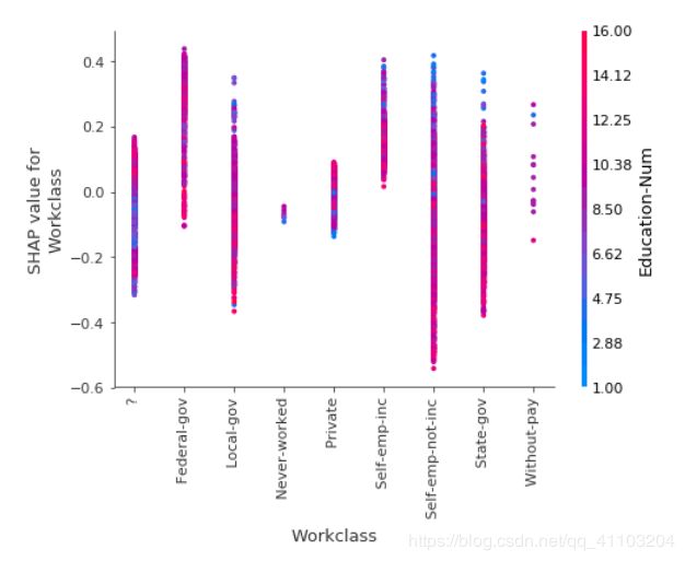
这样就能够正常显示分类变量的结果。也就是说，如果希望后面正常使用shap 的全部功能的话，最好就是在刚开始的时候，我们先把分类变量转成数字形式，也就是OrdinalEncoder 编码。

不过OrdinalEncoder 是否会影响lightgbm 这种树模型的预测结果，这个还不清楚，不过按照树模型的训练方式来讲，应该不会有影响。

在这个例子里，分类变量全都变成了int8类型。

X_train.dtypes

Age               float32
Workclass            int8
Education-Num     float32
Marital Status       int8
Occupation           int8
Relationship        int32
Race                 int8
Sex                  int8
Capital Gain      float32
Capital Loss      float32
Hours per week    float32
Country              int8
dtype: object

参考资料：
https://www.kaggle.com/slundberg/interpreting-a-lightgbm-model?scriptVersionId=3833538
https://github.com/slundberg/shap/issues/254
https://github.com/slundberg/shap
https://github.com/slundberg/shap/blob/master/notebooks/tree_explainer/Census%20income%20classification%20with%20LightGBM.ipynb